Talk:CE1014

JC: General comments: All tasks completed, but your written answers were very brief and lacked detail. Try to expand your explanations and go into a bit more depth on what your results show and their significance.

Theory

Comparing the velocity-Verlet algorithm to the classical solution ($x\left(t\right)=A\cos (\omega t+\varphi )$) of modelling the displacement of a harmonic oscillator as a function of time.

Displacement of Harmonic oscillator as a function of time using classical solution

Energy as a function of time using velocity-verlet algorithm

Absolute difference between Analytical solution and the velocity-Verlet solution for displacement

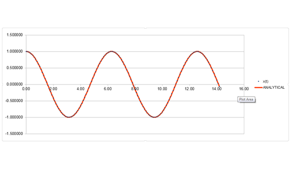
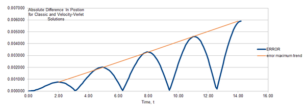
It can be seen that the maximum absolute error between the velocity-Verlet and the classical solution increases linearly as a function of time overall.

Maximum error between values of displacement as function of time for time step of 0.01

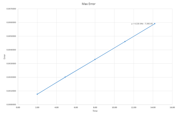
JC: Why does this happen and why does the error oscillate?

What sort of a timestep do you need to use to ensure that the total energy does not change by more than 1% over the course of your "simulation"? Why do you think it is important to monitor the total energy of a physical system when modelling its behaviour numerically?

Energy of Harmonic oscillator as a function of time using velocity-verlet algorithm

The largest timestep possible before the energy increases by more than 1% than the average energy of the system is 0.28. The total energy of the system is kept fluctuating between 1% of the average, as energy in a real system must be conserved and the simulation must model this as closely as possible. The timestep 0.285 can be seen in the graph above and is fluctuating at just above 1% of the average energy.

JC: Good choice of timestep.

For a single Lennard-Jones interaction,$\varphi \left(r\right)=4ϵ(\frac{{\sigma }^{12}}{r^{12}}-\frac{{\sigma }^6}{r^6})$;

• $r_0$ is found where $\varphi \left(r\right)=0$, therefore:

$0=4ϵ(\frac{{\sigma }^{12}}{r_0^{12}}-\frac{{\sigma }^6}{r_0^6})$

${\sigma }^{12}-{\sigma }^6{r}_0^6=0$

${\sigma }^6(r_0^6-{\sigma }^6)=0$

$r_0^6={\sigma }^6$

$r_0=\pm \sigma$

As $r_0>0$ therefore $r_0=\sigma$

• Force at $r_0$:

$F\left(r\right)=-\frac{\mathrm{d}\varphi \left(r\right)}{\mathrm{d}r}$

$-\frac{\mathrm{d}\varphi \left(r\right)}{\mathrm{d}r}=-4ϵ(-12{\sigma }^{12}{r}^{-13}+6{\sigma }^6{r}^{-7})$

When $r=r_0=\sigma$:

$F\left(r_0\right)=\frac{24ϵ}{\sigma }$

• $r_{eq}$ is found where $-\frac{\mathrm{d}\varphi \left(r\right)}{\mathrm{d}r}=0$

$4ϵ(12{\sigma }^{12}{r}_{eq}^{-13}-6{\sigma }^6{r}_{eq}^{-7})=0$

$2{\sigma }^6=r_{eq}^6$

$r_{eq}=2^{\frac{1}{6}}\sigma$

• Well depth at $\varphi \left(r_{eq}\right)$:

$\varphi \left(r_{eq}\right)=4ϵ({\left(\frac{\sigma }{2^{\frac{1}{6}}\sigma }\right)}^{12}-{\left(\frac{\sigma }{2^{\frac{1}{6}}\sigma }\right)}^6)$

$\varphi \left(r_{eq}\right)=-ϵ$

When $ϵ=\sigma =1$

• $\underset{2\sigma }{\overset{\mathrm{\infty }}{\int }}\varphi \left(r\right)\mathrm{d}r$

$=4{[(-\frac{r^{-11}}{11})-(-\frac{r^{-5}}{5})]}_2^{\mathrm{\infty }}$

$=-\frac{699}{28160}\approx -0.0248$

• $\underset{2.5\sigma }{\overset{\mathrm{\infty }}{\int }}\varphi \left(r\right)\mathrm{d}r$

$=-\frac{4391808}{537109375}\approx -0.00818$

• $\underset{3\sigma }{\overset{\mathrm{\infty }}{\int }}\varphi \left(r\right)\mathrm{d}r$

$=-\frac{32056}{9743085}\approx -0.00329$

Number of molecules in 1 mL of water under standard conditions $\approx 3.34$ x $10^{22}$ molecules.

An atom in a cubic simulation box at position $(0.5,0.5,0.5)$, moves along the vector $(0.7,0.6,0.2)$, will end up in position vector $(0.2,0.1,0.7)$ if periodic boundary conditions are applied.

Volume = 2.99 x 10^-25 m^3 The Lennard-Jones parameters for argon are $$\begin{gathered} \sigma =0.34\mathrm{n}\mathrm{m},ϵ \\ / \\ {k}_B=120\mathrm{K} \end{gathered}$$. If the LJ cutoff is $r^{*}=3.2$, what is it in real units? What is the well depth in $$\begin{gathered} {\mathrm{k}\mathrm{J} \\ \mathrm{m}\mathrm{o}\mathrm{l}}^{-1} \end{gathered}$$? What is the reduced temperature $T^{*}=1.5$ in real units?

• distance $r^{*}=\frac{r}{\sigma }$

$r=r^{*}\sigma$

$r=1.09nm$

• energy $E^{*}=\frac{E}{ϵ}$

$ϵ=120k_B$ in J

For kJ/mol, multiply by Avogadro's number $N_A$

$ϵ=0.998kJmo{l}^{-1}$

• temperature $T^{*}=\frac{k_{B}T}{ϵ}$

$T=\frac{T^{*}ϵ}{k_B}$

$T=180K$

JC: All maths correct and nicely laid out. You should show your working for the number of water molecules in 1 ml and the volume of 1000 molecules.

Equilibriation Tasks

TASK: Why do you think giving atoms random starting coordinates causes problems in simulations? Hint: what happens if two atoms happen to be generated close together?

Generating random coordinates for atoms has the potential to place two atoms less than a radius away from each other, in which case the Lennard-Jones potential would not describe the system. This is not a good approximation to real life liquids as the intermolecular forces would not allow atoms that close.

JC: The Lennard-Jones potential can still describe interactions at distances of < sigma, but the repulsive forces generated when particles are placed very close together can make the system unstable and cause the simulation to crash.

The lattice spacing for a number density of 0.8 for a simple cubic unit cell:

$D=\frac{m}{V}$ where $D=$ Number density; $m=$ mass of atom; $V=a^3=$ volume, where $a$ is the side length of the cubit unit cell.

Therefore $0.8=\frac{1}{a^3}$ and $a=1.07722$

Lattice spacing for a face centered cubic lattice:

If $D=1.2$ and $m=4$

$a=1.49380$

For a face-centered cubic lattice with 1000 lattices generated:

4000 atoms would have been created

JC: Values are correct, but you are calculating a number density not a mass density, so m in your equation is the number of atoms in the unit cell rather than the mass.

Meaning of LAMMPS code:

mass 1 1.0 : mass i value; where i = atom type; value = mass of atom

pair_style lj/cut/opt 3.0 : pair_style style args; style = definite style from list (lj/cut corresponds to cut off Lennard-Jones potential with no Coulomb. opt suffix has no effect functionally but means it has been optimized to run faster.); args = arguments used by a particular style (3.0 - cut off point in L-J)

pair_coeff 1 1 1.0 1.0 : pair_coeff I J args - I,J = atom type, coefficients for one or more pairs of atoms interacting with each other

JC: For the Lennard-Jones potential, the coefficients are the values of epsilon and sigma. Why do we use a cut off in the Lennard-Jones potential.

As we are specifying ${\mathbf{x}}_i\left(0\right)$ and ${\mathbf{v}}_i\left(0\right)$, the integration algorithm used will be:

velocity-Verlet algorithm

The value ${timestep} variable is always replaced by 0.001 as this is what the variable is set to at the beginning of the script as:

This saves time when writing the simulation script as if we want to change the timestep in another simulation we would only have to input the value in once; where the variable was being set, rather than having to change the timestep each time is appears in the script. This also reduces the likelihood of mistakes as we won't be able to miss one value which could ruin the simulation.

JC: Correct.

Plots of the energy, temperature, and pressure, against time for the 0.001 timestep experiment:

Energy as a function of time for timestep 0.001

Temperature as a function of time for timestep 0.001

Pressure as a function of time for timestep 0.001

Energy as a function of time for different time steps

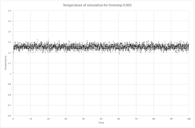
Equilibrium: At time step 0.001, the energy, pressure and temperature all reach equilibrium in a short time of around 0.4 or 40 timesteps.

Choosing timestep: As can be seen from the above graph of energy as a function of time for varying timesteps, the timestep of 0.0025 gives around the same equilibrium value as using 0.001, but the simulation will not take as long as it's a higher value. For the values above 0.0025 the equilibrium energy is dependent on timestep, therefore although the simulation will take less time to run with shorter timesteps, it will not give us the accuracy needed. Therefore 0.0025 is the optimum timestep to choose out of the ones tested here. 0.015 is the worst timestep out of those tested as the total energy does not equilibriate in the time given.

JC: Good choice of timestep and justification.

Running Simulations Under Specific Conditions Tasks

Pressures ,$p$, and temperatures, $T$, chosen for Npt calculations:

$p=$2.75 and 3.0

$T=$1.6, 1.8, 2.0, 2.2 and 2.4

We need to find $\gamma$ so that the temperature is correct $T=\mathfrak{𝔗}$ if we multiply every velocity $\gamma$ .

$\frac{1}{2}\sum _i{m}_i{v}_i^2=\frac{3}{2}N{k}_{B}T$

$\frac{1}{2}\sum _i{m}_i{\left(\gamma v_i\right)}^2=\frac{3}{2}N{k}_B\mathfrak{𝔗}$

Determining $\gamma$.

$\frac{1}{2}\sum _i{m}_i{\gamma }^2{v}_i^2=\frac{3}{2}N{k}_B\mathfrak{𝔗}$

$\frac{1}{2}\sum _i{m}_i{v}_i^2=\frac{3}{2}\frac{N{k}_B\mathfrak{𝔗}}{{\gamma }^2}$

Therefore: $\frac{3}{2}N{k}_{B}T=\frac{3}{2}\frac{N{k}_B\mathfrak{𝔗}}{{\gamma }^2}$

${\gamma }^2=\frac{N{k}_B\mathfrak{𝔗}}{N{k}_{B}T}$

$\gamma =\sqrt{\frac{\mathfrak{𝔗}}{T}}$ , where we have chosen the positive sign of the square root as we do not want the gamma factor switching the direction of the velocities at each timestep.

JC: Good, clear derivation.

Importance of the three numbers 100 1000 100000 in the line - fix aves all ave/time 100 1000 100000...:

100: Use input value this many timesteps.

1000: Number of times to use input values for calculating averages.

100000: Calculate averages this many timesteps

JC: You should explain what these number mean in your own words and/or give and example so that it is clear that you understand them, rather than just copying the definitions from the LAMMPS manual.

For the next line run 100000 means that 100000 timesteps will be taken of 0.0025 therefore a time of 250.

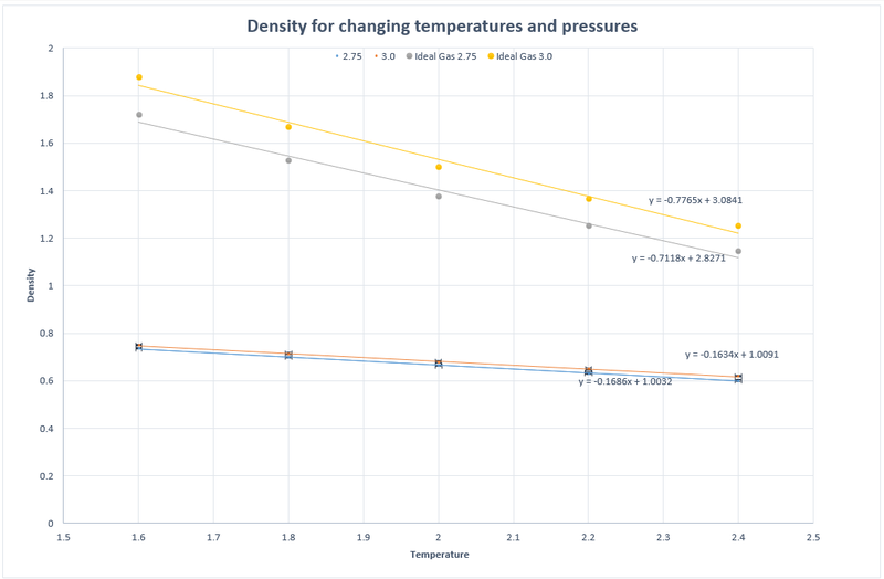
TASK: When your simulations have finished, download the log files as before. At the end of the log file, LAMMPS will output the values and errors for the pressure, temperature, and density . Use software of your choice to plot the density as a function of temperature for both of the pressures that you simulated. Your graph(s) should include error bars in both the x and y directions. You should also include a line corresponding to the density predicted by the ideal gas law at that pressure. Is your simulated density lower or higher? Justify this. Does the discrepancy increase or decrease with pressure?

The simulated density is lower than that predicted by the Ideal Gas Law. This is due to the Ideal Gas Law approximating 0 interactions between particles therefore the particles are able to get closer together in a box of specified volume than in our simulation where we use the L-J approximation which includes intermolecular forces.

The discrepancy increases with pressure.

JC: Would you expect the discrepancy to increase with pressure and how does the agreement between the results change with temperature? Don't fit the ideal gas law with a straight line as you know analytically that the ideal gas law will not give a straight line since density = 1/temperature.

Density as a function of temperature for different pressures

Calculating Heat Capacities

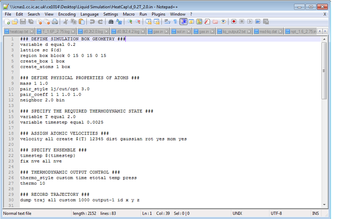
TASK: As in the last section, you need to run simulations at ten phase points. In this section, we will be in density-temperature $({\rho }^{*},T^{*})$ phase space, rather than pressure-temperature phase space. The two densities required at $0.2$ and $0.8$, and the temperature range is $2.0,2.2,2.4,2.6,2.8$. Plot $C_V/V$ as a function of temperature, where $V$ is the volume of the simulation cell, for both of your densities (on the same graph). Is the trend the one you would expect? Attach an example of one of your input scripts to your report.

Heat capacity per unit volume for different densities

The trend is as expected as $C_V/V$ decreases as temperature increases and is consistent with the equation : $C_V=\frac{dE}{dT}$

JC: Why is it what you expected, can you give more of an explanation? What are the curved lines on the graph, give the equations for lines of best fit.

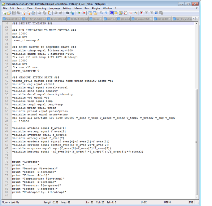
Example of input script:

Script

Script

Radial Distribution Function

Radial Distributions for each phase

At radius 0, the RDF is also 0 as atoms cannot pack on top of each other. The solid data has more peaks indicating a regular structure as the atoms are arranged in lattices. The liquid has less peaks corresponding to increasing disorder, and the gas even more so. At large r, g(r) tends to 1 as it gets closer to the density of the whole system.

JC: Try to be a bit more specific, the liquid has short ranged order (peaks at small r), but no long ranged order, unlike in the solid.

Solid RDF The first three peaks are labeled in the above graph which correspond to the 3 nearest atoms from the origin atom. As the structure is FCC we can see from the image below which spacings the 3 peaks correspond to with value 1, 2 and 3 being 0.975, 1.425 and 1.725 respectively. Therefore the lattice spacing is 1.425, corresponding to the the second peak on the graph and spacing labeled 2 on the image below.

The coordination number for each site is as follows:

1 = 12

2 = 6

3 = 24

Lattice spacing

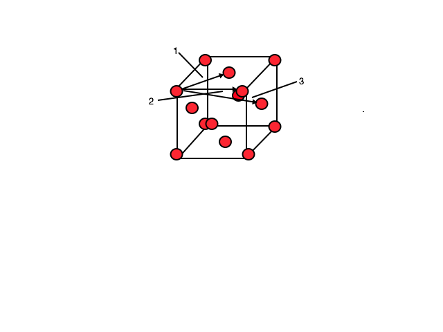
JC: Good idea to include a diagram of an fcc lattice and correct value for the lattice spacing. You could have also calculated this from the first and third peaks and taken an average. How did you get the coordination number, did you plot the integral of the RDF?

Displacement

Plots showing the mean squared displacement as a function of timestep for simulations in different states.

Displacement for each phase

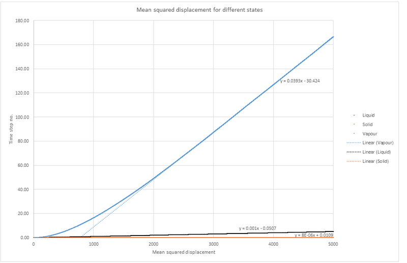
Plot showing MSD for a simulation with 1 million atoms.

Displacement for each phase with 1 million atoms

$D=\frac{1}{6}\frac{\partial ⟨r^2\left(t\right)⟩}{\partial t}$

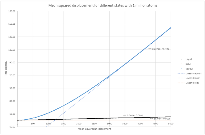
$⟨r^2\left(t\right)⟩=mx+c$ where $mx+c$ is the linear equation from the graphs above.

$\frac{\partial ⟨r^2\left(t\right)⟩}{\partial t}=m$

Therefore $D=\frac{1}{6}m$

Solid simulation: $D=1.33$ x $10^{-6}$

Liquid simulation: $D=1.67$ x $10^{-4}$

Vapour simulation: $D=6.55$ x $10^{-3}$

For simulation with 1 million atoms:

Solid simulation: $D=8.33$ x $10^{-9}$

Liquid simulation: $D=1.67$ x $10^{-4}$

Vapour simulation: $D=6.30$ x $10^{-3}$

JC: Data looks good, what are the units?

Velocity Autocorrelation Function

Evaluate the normalised velocity autocorrelation function for a 1D harmonic oscillator (it is analytic!):

$C\left(\tau \right)=\frac{\underset{-\mathrm{\infty }}{\overset{\mathrm{\infty }}{\int }}v\left(t\right)v(t+\tau )\mathrm{d}t}{\underset{-\mathrm{\infty }}{\overset{\mathrm{\infty }}{\int }}{v}^2\left(t\right)\mathrm{d}t}$

Position of a 1D harmonic oscillator as a function of time: $x\left(t\right)=A\cos (\omega t+\varphi )$

Therefore $v\left(t\right)=\frac{\mathrm{d}x\left(t\right)}{\mathrm{d}t}=-A\omega \sin (\omega t+\varphi )$ and $v(t+\tau )=-A\omega \sin (\omega t+\omega \tau +\varphi )$

$C\left(\tau \right)=\frac{\underset{-\mathrm{\infty }}{\overset{\mathrm{\infty }}{\int }}\mathrm{d}t\sin (\omega t+\varphi )\sin (\omega (t+\tau )+\varphi )}{\underset{-\mathrm{\infty }}{\overset{\mathrm{\infty }}{\int }}\mathrm{d}t{\sin }^2(\omega t+\varphi )}$

$=\underset{T\to \mathrm{\infty }}{\lim }\frac{\underset{-T}{\overset{T}{\int }}\mathrm{d}t\sin (\omega t+\varphi )\sin (\omega (t+\tau )+\varphi )}{\underset{-T}{\overset{T}{\int }}\mathrm{d}t{\sin }^2(\omega t+\varphi )}$

$\underset{-T}{\overset{T}{\int }}\mathrm{d}t\sin (\omega t+\varphi )\sin (\omega (t+\tau )+\varphi )=T\cos \left(\omega \tau \right)-\frac{1}{2\omega }\cos (2\varphi +\omega \tau )\sin \left(2\omega T\right)$

and

$\underset{-T}{\overset{T}{\int }}\mathrm{d}t{\sin }^2(\omega t+\varphi )=T-\frac{1}{2\omega }\cos \left(2\varphi \right)\sin \left(2\omega t\right)$

so

$C\left(\tau \right)=\underset{T\to \mathrm{\infty }}{\lim }\frac{T\cos \left(\omega \tau \right)-\frac{1}{2\omega }\cos (2\varphi +\omega \tau )\sin \left(2\omega T\right)}{T-\frac{1}{2\omega }\cos \left(2\varphi \right)\sin \left(2\omega t\right)}$

$=\underset{T\to \mathrm{\infty }}{\lim }\frac{T\cos \left(\omega \tau \right)}{T}=\underset{T\to \mathrm{\infty }}{\lim }\cos \left(\omega \tau \right)=\cos \left(\omega \tau \right)$

JC: Derivation looks good, but it would be good to show a few more steps in your working, especially the trigonometric identities that you use to perform the integration.

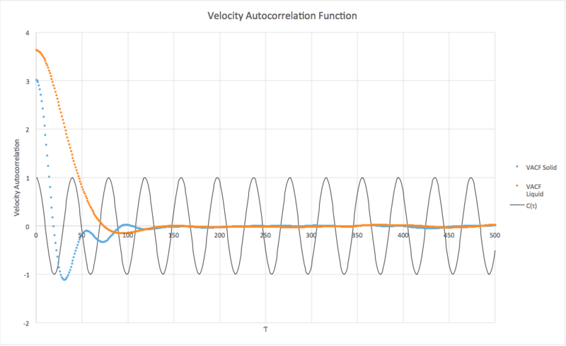
Be sure to show your working in your writeup. On the same graph, with x range 0 to 500, plot $C\left(\tau \right)$ with $\omega =1/2\pi$ and the VACFs from your liquid and solid simulations. What do the minima in the VACFs for the liquid and solid system represent? Discuss the origin of the differences between the liquid and solid VACFs. The harmonic oscillator VACF is very different to the Lennard Jones solid and liquid. Why is this? Attach a copy of your plot to your writeup.

The minima in the graph simulate where atoms have collided. Solid moves very little as lattice structure so D is almost 0 in both cases. The HO is very different as its a approximation and does not take in quantum effects - it is just using classical equations. For our simulation

JC: The simulations are also classical and don't account for quantum effects. The VACF for the solid and liquid decay to zero because of collisions between atoms which randomise the velocities. There are no collisions in the harmonic oscillator.

Liq integer $=119.166$ where $D=39.772$

Solid int = -0.571363169 where $D=-0.190453$

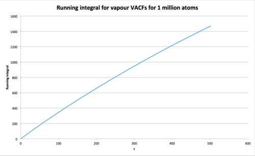
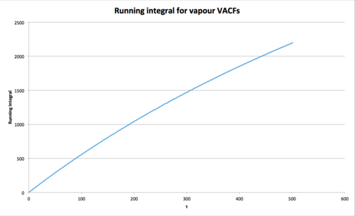
Vapour int = 2197 where $D=732.43$

For 1 million atoms

Liq integer $=123.738$ where $D=41.246$

Solid int $=-0.3745$ where $D=-0.1248$

Vapour int $=1468.85$ where $D=489.617$