This workshop comprises a single 2.5 hour session which serves as an introduction to a technique known as molecular mechanics modelling. The course consists of the following components
ChemBio3D
A Site License for a program system called ChemBio3D is available for you to install on your own computer. This license will expire at the end of August 2015, and this section remains here for the time being only.
What does the ChemBio3D Program Do
The Program is found from the Windows Start menu in the folder ChemBioOffice 2014, as ChemBio3D Ultra 14.0. It loads up with two side-by-side windows. To the right, you will recognise the familiar ChemDraw Window. To the left is a version of the molecule to which three dimensions have been added. Initially, the third dimension is added using very simple rules inferred from the Chemdraw structure drawing, coupled with the stereochemical notation you may have used. This structure can then be refined using a technique called Molecular mechanics.
This defines a mechanical model of a molecule based in essence on Hook's law. This specifies how much energy it takes to distort a spring (in this case a bond or angle) from its equilibrium position. ChemBio3D has built-in force constants for various types of bond (and angle). Together with other terms, this collection is called a force field, and the total energy calculated using this field is called the strain energy.
This energy is then minimised using standard algorithms by adjusting the values of the bond lengths, angles, torsions (and non-bonded terms), producing an optimised geometry. Any given geometry represents only one minimum of potentially many. There is no easy way of finding the lowest minimum of all, often called the global minimum, and you have to use your knowledge of chemistry and molecules to search for this.
One feature characteristic of molecular mechanics models is that once defined, a bond cannot break (Hook's law, a quadratic function, predicts the energy rises to ∞ as the distance increases). This has an advantage: you decide what atoms are connected, by which type of bond, and they remain so! The disadvantage is that reactions cannot be studied using this methodology.
Currently, the ChemBio3D can handle only (some) combinations of the common elements. It does not handle metals and most of the 'left-hand-side of the periodic table.
Using ChemBio3D
Place the mouse cursor in the rhs Chemdraw Window, and sketch your molecule.
Trace over a bond twice for double, thrice for triple.
Use the hash and wedge keys to impart stereochemical information, including stereochemistry at ring junctions.
Use the A item in the Chemdraw menu to change carbons to eg Br, Cl, etc.
Show the configuration of chiral atomic centres by a right mouse click in the drawing area, and from the menu selection that appears, select object and then show stereochemistry. The R/S notation for each centre appears. Check it's correct by focusing on the lhs 3D window, select the rotate icon (to the right of the little hand in the second row) and orientating the lowest priority group at any given chiral atom away from your viewpoint, assign the priorities of the remaining three groups.
Use the templates to deposit fragments into the ChemDraw window. Learn how to join fragments together by either atoms or bonds.
Once the basic drawing is complete, focus on the 3D window.
Use icon labelled 3 to set mouse-driven rotation of the molecule. Inspect it in 3D.
To move an atom (for example to change a hydrogen from pointing up to pointing down) firstly select it using icon 2, then set move using icon 5, then drag the atom from where it is, to where you want it to be.
Once you have a structure that is approximately correct, its time to invoke the Molecular-mechanics based tidying of the 3D coordinates. From the top menu, invokecalculations/MM2/Minimise energy. This will take about 2-20 seconds. A total (steric) energy is printed in the information box at the bottom (in kcal/mol). Record this energy.
Using the editing buttons, make appropriate changes (such as moving atoms, or, in the Chemdraw Window, changing the stereochemistry), and repeat the minimisation. Compare the two energies, and decide on that basis which isomer is the most stable.
Hint1: If you want to move an atoms (say to change a conformation from chair to boat), firstly delete on the hydrogens on it, then move it, then (via structure/rectify) re-add the hydrogens, and finally reminise. If you do not remove the hydrogens first, the moved atom is quite likely to spring back to where it originally came from.
Hint2: To change the conformation about a single bond by adjusting the dihedral angle, proceed as follows:
Using the atom select tool (arrow, first icon on left above) and (pressing the shift key after the first selection), select the four atoms defining the dihedral (for example, Br, C, C, Cl).
Pull down menu Structure/Measurements/Display dihedral measurement' produces a measurement box. In the box labelled Actual, type the value of the dihedral you want to set and press the return key. It should "take", and the new conformation will be displayed.
Re-minimise the conformation
Hint3: To change the configuration at a single carbon centre, first select the carbon using the atom select tool, then pull-down structure/invert. If you select the whole molecule, then the enantiomer of that molecule is produced.
To start a new molecule, use the capture tool (in Chemdraw) to select all of what you have, press delete, and start again.
Avogadro
This is a general purpose 3D molecular modelling program, available as open source as version 1.1.[1] Bugs commonly encountered by students are documented here Get Avogadro from here. It is available for Windows, OS X and Linux.
Using the program
The main menu functions as follows. The most important tools are in bold.
Ensure that the button labelled Tool Settings is toggled blue. This ensures that the tool settings appear on the left
The draw tool. Use this to draw new atoms (carbon by default), dragging out a bond from an existing atom and releasing the mouse to drop a new atom.
To close a ring, drag to the ring-closing atom and release (the hydrogens at the closed bond will be automatically removed).
To delete atoms, click on them whilst pressing the right-mouse-button.
To move (drag) atoms, place the mouse pointer on them, and drag to a new destination.
For charged atoms (i.e. R-O(+)=C ), just specify the bond order and ignore the charge.
Bonds can be created between two existing but non bonded atoms by specifying a bond order (single by default) and dragging the mouse between them.
A right-mouse-click on a bond will remove it.
The navigation tool, used to rotate and manipulate the structure
Bond centric manipulation tool. Easier used than described!
Manipulate (move) atoms. Use this to correct stereochemistry, alkene configuration, etc.
Selection tool.
Autorotation tool. Rotates the molecule according to a vector drawn with the mouse cursor.
Energy optimisation tool. Use to calculate a molecular mechanics energy.
use the following settings: Force Field=MMFF94s, Algorithm=Conjugate gradients
Toggle 'Display Settings' on (the button will be blue) and tick Force in the display types. This shows the forces on each atoms during optimisation, which is complete when all the forces have vanished.
Click start to obtain an energy. The optimiser remains in effect until you toggle to stop in order to edit the molecule, using e.g. move atoms (otherwise the auto-optimisation will rubber-band the atom and immediately return it to its start position).
Measurement tool. Use to calculate lengths, angles and dihedral values.
Strategy
The easiest way to create a molecule is to sketch it first in ChemDraw, save this as a .cdxml chemdraw file (do NOT use the older .cdx format, which crashes Avogadro), and then either drag-n-drop this file into the Avogadro viewing window, or simply open from within Avogadro, where it will be converted to an ~3D coordinate model of the molecule. You may have to correct stereochemistry by dragging atoms into the correct stereochemical position.
To use Avogadro to start other types of calculation, use the Extensions menu item to create a job file for other programs (e.g Gaussian).
Avogadro can also be used to read the outputs of other programs (e.g. Gaussian) and to display computed properties (vibrations, orbitals, etc).
Follow ups to this Course
The molecular mechanics procedure is quick and simple, but not always accurate. Different molecular mechanics force fields also vary in their accuracy.
A proper molecular model must also take into account electrons, as noted above. But solving the necessary equations takes much more computer time. In the accompanying symmetry course in 2nd year, you will be shown how to use a programs such as Gaussview. This is the front end to a Quantum mechanical modelling program Gaussian, which you will use in earnest in the third and fourth year, along with courses which deal with the theory and practice in much more detail.
Further Documentation, Reading and Viewing
Ghemical Manual gives more advanced options, but be aware it relates to an earlier version of Ghemical.
Third year modelling lab on Inorganic Chemistry, including three advanced individual projects on Mo(CO)4L2, boron based acids and Gold interactions with Water.
A local third year course on organic molecular modelling with a number of more elaborate case studies illustrating the application of molecular modelling.
The grand Daddy of all molecular models, invented at (what was to become) Imperial College around 1860, and now in the archives of the Royal Institution. These models are the source of the familar colour scheme now used, i.e. Hydrogen=White, Oxygen=Red, Nitrogen=blue, etc.
Another father of molecular modelling, but only on paper!, also achieved in 1861. Loschmidt constructed these models in the same sense that Watson and Crick did for DNA, as proposals, and not representing structural proof in any way.
For an interesting way of presenting scientific genealogies of scientists, see J. Andraos, Scientific genealogies of physical and mechanistic organic chemists, Can. J. Chem./Rev. Can. Chim., 2005, 83, 1400-1414. DOI:
The preception of the 3D character of many molecules can be enhanced by viewing using stereoscopic systems. One such system is available for student use, and lecture theatre C is equipped with stereoscopic projection.
Submitting more accurate calculations to the Departmental HPC Cluster
Export from Ghemical
The Chemistry department runs a HPC (high performance computing) system, which be used to run more time consuming calculations than is possible interactively on a single e.g. laptop or desktop computer whilst sitting in front of it.
One far more reliable and quantitative way of modelling a molecule is to subject it to quantum mechanical modelling using Density Functional theory. In practice, this is implemented here using a program called Gaussian 09. The procedure to submit such a job is as follows:
Creating an Input file
After you have optimised your sketched molecule using Ghemical, as described above, right click in the black display window. This will produce the floating menu, from which you select file and then Export. Select Gaussian 98/03 Cartesian Input for the type and type a name for the file (make sure that the name of the file ends with .gjf). It will be saved in your H: drive by default.
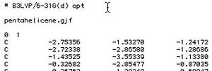
Typical Gaussian inputThe file will have to be edited before it can be submitted. You can do this either with Gaussview as the program, but a much simpler method is to open the file (pentahelicene.gjf in this example) using eg the Windows Wordpad editor. This is invoked simply by double clicking on the file. Remove any existing lines starting with % or # and replace them with one of the following single lines (the second example also results in the vibrational frequences and from these the entropy being computed, and hence the zero-point and free-energy corrected value, ΔG). This latter option will take significantly longer however.
# B3LYP/6-31G(d) opt
or # B3LYP/6-31G(d) opt freq
to produce a file that looks like the one shown on the right.
For a molecule the size of e.g. pentahelicene, the calculation will take about 4-5 hours overnite. If for some reason, your molecule is taking longer, you can always reduce the size of the basis set to e.g. B3LYP/3-21G*, or submit the job on a Friday, when it will have the entire weekend available to it. If you want greater accuracy (but for longer computing time), try e.g. # B3LYP/cc-pVTZ opt freq.
Submitting the Input file
Create a new jobYou will have to login as yourself. You can submit as many jobs as you wish through this mechanism, but you must prepare the input (.gjf) file for each first. The SCAN operates during the period 23.00-07.30 overnight. If a job is not completed during this period, it will be scheduled to run again (from the beginning) the next night. For this reason, you should only schedule jobs that can complete in an 8 hour window. In practice this means submitting molecules only a little bit larger than pentahelicene.
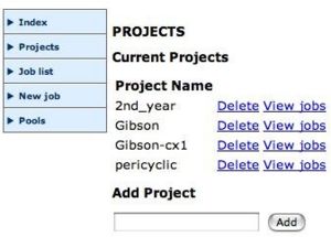
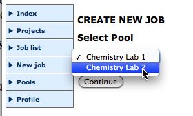
Create a projectSelect a poolAfter you are logged in you should organise your jobs by project. Create a suitable new project, then select New job, the Application (currently only Gaussian) the Project, and press continue.
Upload your input fileYou now have to find the Gaussian input file, as prepared above. You should Browse to drive H: to find this file. Add a description which will help you identify the job.
The Chemistry Condor PoolThe job will be added to your list of jobs, andyou can view its status (but this depends on there being a vacant machine in the Condor pool).
Viewing the outputsWhen the job has completed, click on the Job List link. This will show all available outputs. Download the program Log file (this will help you chart whether the calculation was successfull) or the Gaussian Formatted Checkpoint file onto the desktop of the computer you are using, and the file should open up Gaussview, where the molecule can be viewed and checked. You can use the latter file to e.g. plot molecular orbitals for the molecule, view vibrational modes, etc. Full details of these procedures are described in the Gaussview manuals.
Archiving the output into a digital repository
Depositing an entry in DSpace
A very recent innovation is the Institutional digital repository, a resource for permanently archiving calculations, spectra and crystal structures. You can get a flavour of this by archiving your own calculation in the SPECTRa digital repository. To the right of the Portal display is a link termed Publish. If you click on this, and the calculation is actually in a state to be published (it may for example have failed for some reason) then appropriate metadata for the calculation is collected, and the collection deposited into the repository. From here, it can be retrieved in future.
About this wiki: Opencourseware
This course is presented as a wiki. This differs from conventional hand-outs or web pages in several aspects.
Anyone (who has a valid Imperial College login and password) can edit it, for the purpose of correcting errors, clarifying ambiguities, and even adding more examples, or references to existing examples. However, this activity is not anonymous; you can see who has done what by inspecting the history of the article. If you are considering making changes, go read these rules first.
You may notice that some terms appear in red. This is because the original author has enclosed the term thus: [[red]], acting as a suggestion or hint that someone may wish to pick up this term, and expand it into something informative. If you think you can add something helpful to others, please go ahead: click on the red section and starting editing! If the result contains inaccuracies, someone may come along and correct them. If you are dubious that this scheme works, just go visit Wikipedia. The idea behind this is that we produce joined up courses and not just isolated islands of information and knowledge.
You can also hit the edit button if you want to find out how any particular effect is achieved. You do not have to actually change anything.
This is an experiment! If you have any comments on the experiment, or suggestions for improvements, go instead to the discussion page and say something there. Do however remember that anyone in the world (!) can see this (it is opencourseware, go read this stimulating and provocative view of how knowledge may be owned and disseminated in the future), so remember not to write anything inappropriate. You cannot do so anonymously!