Rep talk:FabianThomasThirdYearLiquidFlowSimulation

Overall: Good attempt at the lab although the VACF was not attempted. Be careful not to become too colloquial in your writing and read through to check for grammar. Your style is pretty good apart from the grammar and sometimes vague statements - keep it up and read more before your MSci proj, it helps :^) Mark: 68/100

Abstract

Not a bad attempt at writing an abstract - hardware, unless it's revolutionary, doesn't need a mention aka HPC.

Lennard-Jones simulations of solids, liquids, and gases were run through LAMMPS on the imperial HPC service. How number density varied against temperature and at different pressures, radial distribution functions of L-J solids, liquids, and gases, Mean Squared Displacements, Diffusion coefficients, and the variation of heat capacity with temperature were investigated in order to understand more about phase properties, and specifically those that can be modelled using a L-J simulation. For the equation of state, number density increased with pressure, but was inversely proportional to an increasing temperature. Heat capacity was determined to be inversely proportional to temperature due to a change in density of states for a fixed NVT ensemble. The radial distribution function allowed for analysis of solid, liquid, and gas simulations of 3375 atoms and allowed for the probing of the structure of each phase, along with details about the co-ordination spheres and numbers of nearest neighbors. Diffusion coefficients were found using the Mean Squared Displacements gram not capitalised for solids, liquids and gases, along with simulations with one million atoms for each phase as well, with values for $D$ of$-1\times 10^{-17}$,$1.1\times 10^{-10}$ and $$\begin{gathered} 3.61\times 10^{-9} \\ {m}^2{s}^{-1} \end{gathered}$$ for the solid liquid and gas phases. tick

Introduction

Very good introduction Fabian - hit the nail on the head :^) Phase changes occur every day in daily life, and are common place in the world around us. From boiling water to be used in cooking or in steam generators to produce electricity, to instant heat packs, where sodium acetate is super cooled, and upon perturbation instantly raises the pack’s temperature significantly to its freezing point at 54 degrees. These are all every day examples of how phase changes are used and how research into phase changes can provide new avenues for products and areas of research such as new instant-heat pack materials, all based on previous phase change research.

Phase change materials; not unlike sodium acetate, is a large area of research today. Materials capable of storing large amounts of energy through phase changes such as the solid to liquid transition or solid to solid transitions, with applications such as improved solar cell energy storage, and materials able to change state for useful purposes in textiles these simulations carried out can further progress phase-change transition research, and can be used to go on to model more complex systems for use with this research.

Modelling theses systems using L-J simulations provides a fast and easy method to compute the phase change temperatures, order, and structure of the phases transitioned through. Thus simplifying the need to synthesise the molecule beforehand to view the properties of the system. Some of the systems with the largest heat of fusion are systems such as Lithium or water, which are very easily simulated through L-J models and provide an excellent way to probe the phase diagrams of these systems. The ease of determining the crystal structure of solids, is very largely beneficial for the phase change materials, as it allows for easy categorisation of the solid phases, such as ice which has over ten different solid crystalline phases depending on the pressure and temperature of the system, which is modelled accurately and quickly using an L-J simulation through use of radial distribution functions. Heat capacity measurements of phases are of a large interest in phase-change materials as materials with large heat capacities coupled with a large latent heat of fusion allows for the storage of very large amount of energy in a small amount of solid. But all these simulations lead to further questions, how far can L-J simulations go in helping to discover phase change materials, and how accurately can the simulations predict real heat capacities, structures and transitions of unmade molecules?

Methods

A good computational methods section should be structured model, params, forcefield, params. Then describe what you did with this model. Not bad though.

All simulations were run as Lennard-Jones systems through the Imperial College HPC facility using the LAMMPS runtime option, with all graphs and respective data produced and analysed using Origin Pro . Equation of State simulations were run using an NpT ensemble. Using dimensionless L-J reduced units , pressures $p^{*}$ of 1.8 and 2.6 were used, along with temperatures above the critical temperature $T^{*}$ = 1.5 of 2, 2.5, 3, 3.5 and 4. A timestep of 0.0025 was used, as it was found in the earlier stages of the experiment to be as accurate as a timestep of 0.001, but would run the simulation 250% faster in comparison. As it was a liquid that was to be simulated, a simple cubic lattice was used for the simulation.

Heat Capacity simulations were run at ${\rho }^{*}$ = 0.2 and 0.8, and $T^{*}$ = 2.0, 2.2, 2.4, 2.6, 2.8 in L-J reduced units. A simple cubic crystal was melted under microcanonical NVE conditions. As heat capacity, shown below, is directly proportional to the variance of energy of the system if temperature is held constant, after melting, the system was put under an NVT ensemble to hold the temperature constant but allow the energy to vary.

$C_V=\frac{\partial E}{\partial T}=\frac{\mathrm{V}\mathrm{a}\mathrm{r}\left[E\right]}{k_B{T}^2}=N^2\frac{⟨E^2⟩-{⟨E⟩}^2}{k_B{T}^2}$

Where $C_V$ is Heat Capacity, $\mathrm{V}\mathrm{a}\mathrm{r}\left[E\right]$ is the variance in Energy, $k_b$ is Boltzmann's constant, $⟨E^2⟩$ is mean squared energy, ${⟨E⟩}^2$ is mean energy squared, and $N^2$ is the number of atoms in the simulation squared.

A factor of $N^2$ is added to the equation, as LAMMPS divides all energies output by the number of particles in the system, therefor giving $\frac{E}{N}$ for any value of $E$ measured. Using this equation, the heat capacity was found and $\frac{C_V}{V}$ was plotted against $T^{*}$ to view how the heat capacity varied with respect to temperature.

Using VMD software , the radial distributions functions for the solid, liquid, and vapour phases of a L-J fluid were calculated, setting selection 1, and 2 to ‘all’, and delta r to 0.05. Using these plots the co-ordination sphere radii and numbers of the solid, liquid, and vapour phases were determined.

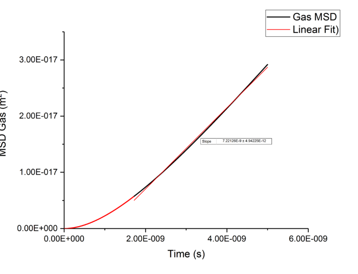
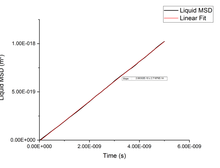
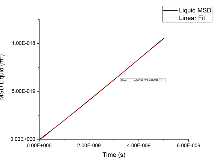
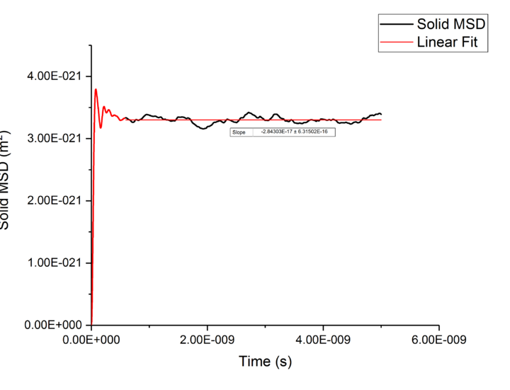
Using the equation $D=\frac{1}{6}\frac{\partial ⟨r^2\left(t\right)⟩}{\partial t}$ and the relationship between D and Mean-Squared Displacement $⟨(x(t)-x_0{)}^2⟩=2Dt$, $D$ was calculated for solid, liquid, and vapour phases by extracting the gradient from the plot of Mean-Squared Displacement against time, giving a gradient of $2D$.

Results and Discussion

Equation of State

Figure 1: A plot of average density against average critical temperature of the system with standard error error bars

From figure 1, we can see that number density $\frac{N}{V}$ is inversely proportional to $T$. This can be rationalised by looking at the results of the L-J reduced gas law $\frac{N}{V}=\frac{p}{T}$

The discrepancies between the idealised and simulated number density results can be attributed to the simulation being non-ideal. The basis of a L-J system is that the particles interact with each other, with a short range repulsive term, and a longer range attractive term. The ideal gas law however, assumes that there are no interactions between particles and thus, due to the short range highly repulsive term, the particles are further apart than in a system with no interactions and therefore the number density of the simulated systems are lower than their idealised counterparts.tick

As the temperature is increased, the kinetic energy of the particles increases leading to an increase in the average distance between particles in order to reduce repulsions between particles to a minimum. This can be seen in Charles’ Lawː

$\frac{N_1}{T_1}=\frac{N_2}{V_2}$

As the temperature is increased to $T_2$, $V_2$ must increase, thus leading to a decrease in number density. As the particles are further away from each other on average, the particles interact with one another less, and so become more ‘ideal’, reducing the difference between the simulated result and the gas law result.tick

This result is the opposite for lower temperatures. As the temperature is reduced, so is the kinetic energy, and therefore the particles are less able to overcome the attractive and repulsive forces between them. This leads to larger interactions between the particles due to their increased proximity to each other, and so simulated results deviate from the gas law more at lower temperatures. From Charles’ Law again, we can see that the volume of the cell will decrease as temperature decreases, and so number density will increase at lower temperatures.tick

From the graphs, we can see that, at higher pressures the deviations from ideality are larger than that of a lower pressure simulation. This arises from the fact that at higher pressures, the number density is higher due to decreased cell volume, leading to decreased distances between particles and therefore increased interactions between them as they collide with each other more frequently. This increase in interactions between particles leads to a large deviation from ideality and so a larger difference between simulated and ideal law data for higher pressures. tick, what about the variation of density with temperature?

Heat Capacity

Figure 2: A plot of $C_V/V$ against $T*$ for two different densities

Figure 3: An image of a sample of the script used for one of the heat capacity calculations

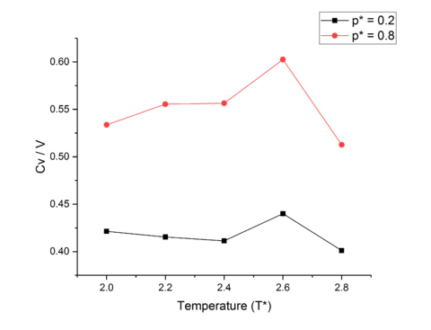
Heat capacity defined in the equation below, varies directly with the variance in energy of a system held at constant temperature, but is essentially a measure of how easily a substance can be heated up. Thus, a substance with a larger heat capacity will require more energy to heat up than one with a lower heat capacity.tick

$C_V=\frac{\partial E}{\partial T}=\frac{\mathrm{V}\mathrm{a}\mathrm{r}\left[E\right]}{k_B{T}^2}=N^2\frac{⟨E^2⟩-{⟨E⟩}^2}{k_B{T}^2}$

The odd relationship between $\frac{C_V}{V}$ and temperature $T^{*}$ can be described through use of the equipartition theorem and the Boltzmann Distribution in part!

The large jumps in heat capacity seen in both data sets at $T^{*}=2.6$ can be explained through phase changes. As the particles simulated are totally symmetric there are no extra degrees of freedom to be reached through an increase in temperature as only translational modes are active through equipartition theorem, therefore the jump in heat capacity must be due to a phase change. tick Assuming a second order phase transition; as an NVT ensemble is used, and in a first order transition density is discontinuous which is impossible for a system with fixed $N$ and $V$, Heat capacity rises to infinity until after the transition has been completed, after which it lowers again, which can be seen at $T^{*}=2.8$, due to thermal energy needing to be expended in order to complete the phase transition. tick, ok good

The decrease of heat capacity with temperature increase excluding phase changes, can be explained through the Density of States. Similar to the anharmonic oscillator model for electron excitation for an atom or particles where as the energy levels are increased, the spacing between the levels decrease, as the temperature of our system is increased the spacing between energy levels contracts, and thus the higher energy levels come down in energy and become more accessible. This leads to more modes available for promotion in the system, thus ease of promotion of an atom increases, leading to a reduced energy needed to promote and atom and so heat capacity decreases with temperature. tick, good

This can be viewed form a different angle with the Boltzmann Distributionː

$\frac{N_i}{N}=\frac{\exp (-E_i/kT)}{\sum _j\exp (-E_j/kT)}$

For a specified energy gap, the higher in energy the energy state is, the less likely it is to be populated. If the energy gap is decreased, higher energy states are more likely to be populated, and are therefore more easily reached, and thus the ease of promotion is increased for a decrease in energy gap between states and so heat capacity falls.tick

Structural Properties of the Radial Distribution Function

Figure 4: ft1015G(r).png

Figure 4: ft1015G(r)N.png

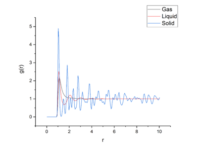
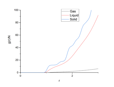
Using VMD the RDFs for a solid, liquid, and gas were found and investigated.

The Radial Distribution Function, RDF, describes for a central particle how density varies as a function of distance $r$. The RDF can be used to find the co-ordination spheres of solids, liquids and gases, along with the distance each sphere lies from the central particle.

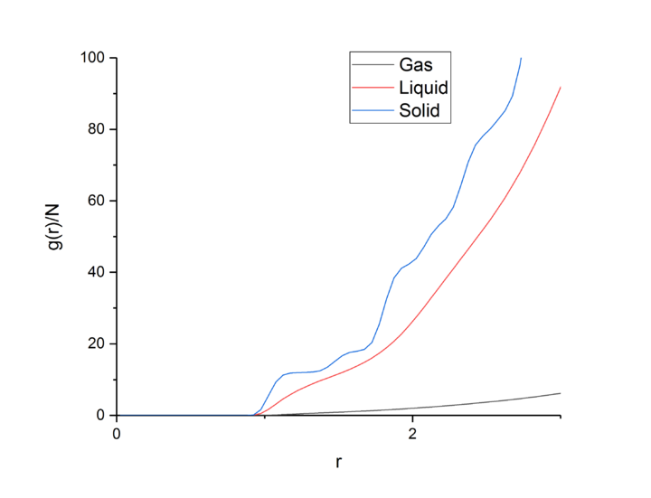
Integrating the RDF gives the number density RDF, which allows users to find out how many particles lie within each co-ordination sphere, and when used in conjunction to the normal RDF, the structure of that phase.tick

Looking first at the RDF for the solid, the large peaks relate to particles being found at that distance from the central atom. These peaks relate to the co-ordination spheres around the atom in the solid phase. The peaks are sharper than the other phases due to the crystal structure of the solid phase and that the particles are fixed in place inside the lattice. Because of the crystal structure and it’s short- and long-range order, the peaks are sharp due to distinct spheres of co-ordination found at each distance. Looking at the first three peaks, these relate to the first three co-ordination spheres or nearest neighbours of particles around the central atom. The troughs in the RDF relate to the empty space between the co-ordination spheres and lack of particles between the spheres. Looking at the first three peaks in the RDF and number integrated RDF, we can say that the first three co-ordination spheres contain 12, 6, and 24 atoms respectively. tick

r	Integrated g(r)	Co-ordination Number
1.175	11.85813	12
1.675	18.44288	6
1.975	42.26256	24

The lattice spacing is the distance between repeat lattice cells and is present in systems with repeating units, and therefore repeating lattice cells. For the FCC lattice in the solid case, the lattice spacing was 1.175 in L-J reduced units. tick

The liquid phase in comparison to the solid phase has a highly reduced order due to the lack of long range order and rigidity in the liquid phase, but more order than the gas phase as one can see in the increased amount of peaks that the liquid phase has in comparison to the gas phase which shows more co-ordination spheres in the liquid phase. As liquid particles are not held tightly in place, but can vibrate and move, the co-ordination peaks are broad due to the fact that the particles are slightly spread out across the co-ordination shell as they are bound, but not tightly. This peak occurs around $r=1$, with further co-ordination shells smaller than the closer shells as the short range order of a liquid breaks down at longer range. The troughs, similarly to the solid are due to no particles being in-between the shells and their atomic neighbours.tick

The gas phase has the least order out of the three phases examined. This is easily seen through there being phraseology like this is a bit colloquial only one peak on the RDF in comparison to the other phases. This peak relates to the very weak attractive forces between gas particles, and their nearest neighbours, effectively leading to one singular diffuse co-ordination sphere, which can be seen by the broadness of the peak. After the first coordination, there is no order relating to the central particle, and so the RDF falls to one after the peak, showing an equal likelihood of finding a gas particle at any distance after the co-ordination sphere, which further emphasises the lack of order in the gas phase.tick

For all phases the RDF is zero until the first co-ordination sphere or right before. This is due to the width of the atoms in the simulation and how the atoms cannot overlap due to the strong repulsive forces. This leads the first particles to be detected by the function at the first co-ordination sphere.tick

Dynamical Properties and the Diffusion Coefficient

Figure 4: A plot of MSD against time for the gas phase

Figure 5: A plot of MSD against time for one million atoms in the gas phase

Figure 6: A plot of MSD against time for the liquid phase

Figure 7: A plot of MSD against time for one million atoms in the liquid phase

Figure 8: A plot of MSD against time for the solid phase

Figure 9: A plot of MSD against time for one million atoms in the solid phase

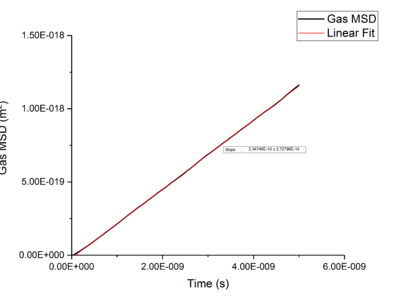
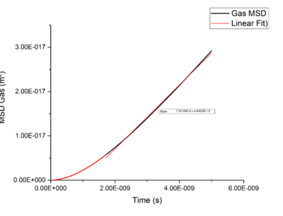
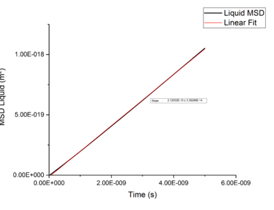
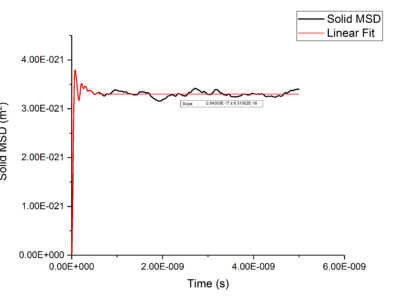
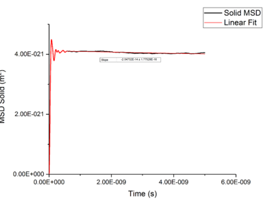
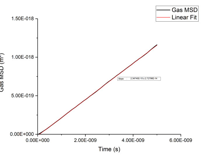
Using Mean Squared Displacement, MSD, in an NVT ensemble, one can determine the diffusion coefficient $D$. MSD is with ? bit unclear, respective to a reference position, the deviation of the position of a particle from said point over time, and can be measured through single particle tracking via photon scattering .

The diffusion coefficient $D=\frac{1}{6}\frac{\partial ⟨r^2\left(t\right)⟩}{\partial t}$$D$ is directly proportional to MSD as shown below in the equation:

$MSD=⟨(x(t)-x_0{)}^2⟩=2Dt$

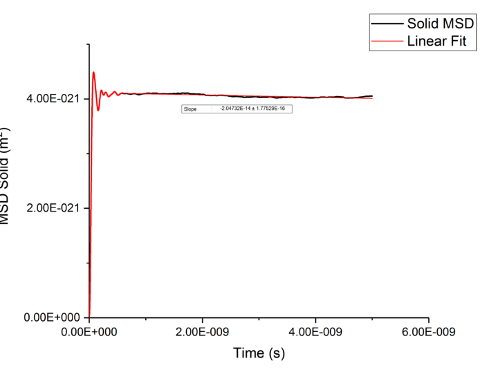
Plotting MSD against time, gives a graph with a gradient of $2D$ and therefore a diffusion coefficient equal to $\frac{gradient}{2}$. These plots can be seen in figures 4-9 for solid, liquid and gas phases, along with plots of data given to us of those phases with one million atoms. If data points were not used in the linear fit of a graph as they did not follow the linearity expected for the gradient were masked and are shown in red on the plot.

Diffusion Coefficient

Phase	Simulated plots / m^2 s^-1	one million atoms plots / m^2 s^-1
Gas	1.17E-10	3.61E-09
Liquid	1.03E-10	1.1E-10
Solid	-1.4E-17	-1E-17

Looking at each phase individually and the two plots associated with them. what? Needs to ensure you maintain the flow and importantly the subject and object of sentences! Starting with the gas phase we can see that for our simulated data diffusive rates are reached immediately and stay constant throughout the simulation as there is little to no order in gas phases which was established by use of the RDF function earlier. However, for the one million atom simulation, the rate of diffusion is not initially constant but rises as the simulation progresses until system reaches equilibrium and $D$ stabilizes. Thus for the one million atoms plot data points outside the linear region were excluded, as shown in the graph.tick

Rates of diffusion for liquids were lower than that of gases, which is to be expected due to the short range order shown in the RDF functions, thus diffuse more slowly to keep the short-range order intact.tick

Values of $D$ for the solid were extremely small to the point of there being no diffusion occurring in solids. This can be explained by the highly ordered structure which only allows particles to vibrate about a fixed point, this is confirmed through RDF calculations above, with the large change in diffusion coefficients are the start of each simulation due to the system reaching equilibrium. Diffusion will only be able to occur in from a solid phase if a phase change occurred and thus diffusion would occur through a different phase.tick

A change in value of $D$ for the larger one million atoms in comparison to our own simulations was expected as these larger simulations are likely to be more accurate and precise due to the larger amount of averaging that is able to occur, and the larger amount of atoms lowers microscopic effects as the system move into the macro scale.tick

Conclusion

Be careful write correct conclusions. Also go through your writing careful - there are a few grammar mistakes throughout and never use the active tense!

Through the successful modelling of a L-J system above the critical temperature, the equation of state was found at two different pressures. Number density was found to increase with pressure due to the increased repulsions between particles because of the increased number of collisions, while also found to be inversely proportional to temperature, as at higher temperatures the particles moved further apart, thus lowering the interactions between them and so lowering the number density, this was reinforced using Charles’ law. Deviations from an ideal gas were seen as the L-J system allows for attractive and repulsive forces between the particles, but at higher pressures the difference from ideality was larger due to the increased density of the particles leading to more interactions between them, thus straying from the ideal gas postulates.

It was found that Heat capacity was inversely proportional to temperature not true! due to the change in density of states associated with an increase in temperature. The increasing of the density of states, and thus the lowering of energy of the higher energy levels allowed for more available energy states for promotion to, and so easier promotions of particles, thus leading to a lowered heat capacity due to the increased ease of promoting a particle to a higher energy state. A peak in the heat capacity seen at $T^{*}=2.6$ was seen due to a change in phase with the heat capacity reaching infinity until the necessary amount of thermal energy had been input to the system.

The radial and integrated radial distribution functions were successfully used to model the co-ordination spheres of a solid, liquid, and gas, along with numbers for the nearest neighbours, and information on the order and structure of each phase. The gaseous phase was found to have no long range order, and only a single co-ordination shell thus leading to extremely short range order, with a broad peak suggesting a diffuse shell. The liquid phase was found to be more ordered than the gaseous phase due to the increased number of three co-ordination shells, leading to short range, but similarly to the gas no long range order in the phase. The peaks were also broadened, suggesting slightly diffusive co-ordination shells. Solids were found to be highly ordered in structure, with long range and short range order due to its crystal structure. Peaks were sharp due to the set spacings between particles, and the fact that the particles can only vibrate around their fixed positions, not move like in a liquid or gas. The co-ordination of the solid was found to be 12, 4, and 24 in the first three co-ordination shells respectively, along with a lattice spacing of 1.175.

Diffusion coefficients for solids, liquids, and gases were also found using the relationship between MSD and $D$. Solids were found to have an almost zero diffusion gradient, while liquids and gases were much higher. Data for 1000000 atoms simulations for each phase were received and plotted, leading to more accurate results for $D$, which agreed with the values of $D$ received from the simulations of 3375 atoms completed by us.maintain passive voice..

Introduction to molecular dynamics simulation

Numerical Integration

TASK: Open the file HO.xls. In it, the velocity-Verlet algorithm is used to model the behaviour of a classical harmonic oscillator. Complete the three columns "ANALYTICAL", "ERROR", and "ENERGY": "ANALYTICAL" should contain the value of the classical solution for the position at time $t$, "ERROR" should contain the absolute difference between "ANALYTICAL" and the velocity-Verlet solution (i.e. ERROR should always be positive -- make sure you leave the half step rows blank!), and "ENERGY" should contain the total energy of the oscillator for the velocity-Verlet solution. Remember that the position of a classical harmonic oscillator is given by $x\left(t\right)=A\cos (\omega t+\varphi )$ (the values of $A$, $\omega$, and $\varphi$ are worked out for you in the sheet).

TASK: For the default timestep value, 0.1, estimate the positions of the maxima in the ERROR column as a function of time. Make a plot showing these values as a function of time, and fit an appropriate function to the data.

TASK: Experiment with different values of the timestep. What sort of a timestep do you need to use to ensure that the total energy does not change by more than 1% over the course of your "simulation"? Why do you think it is important to monitor the total energy of a physical system when modelling its behaviour numerically?

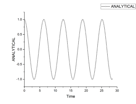
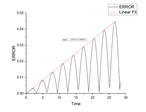
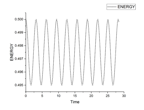
The total energy of a classical harmonic system is given by $\frac{1}{2}m{v}^2$ and $\frac{1}{2}k{x}^2$ for the kinetic and potential energies respectively. Combing these give the total energy of the system which should be a constant for an isolated system as no energy enters or leaves the system. A time-step value of 0.2 s gives a maximum difference in energy of 1% of the total starting energy, and so ensures a good approximation to realistic behavior. The Velocity-Verlet algorithm will have fluctuations in the total energy of the system as it is only an approximation through a Taylor-series expansion, however, minimizing these fluctuations provides a more accurate simulation and therefore for a physical system would provide more accurate thermodynamic properties of the system. Decreasing the time-step, and so decreasing the energy fluctuations will provide more accurate results at the cost of increased simulation time needed for the same time frame of a system, and so is a trade-off between time and accuracy for the simulation.tick

Atomic Forces

For a single Lennard-Jones interaction, $\varphi \left(r\right)=4ϵ(\frac{{\sigma }^{12}}{r^{12}}-\frac{{\sigma }^6}{r^6})$, find the separation, $r_0$, at which the potential energy is zero. What is the force at this separation? Find the equilibrium separation, $r_{eq}$, and work out the well depth $(\varphi \left(r_{eq}\right))$. Evaluate the integrals $\underset{2\sigma }{\overset{\mathrm{\infty }}{\int }}\varphi \left(r\right)\mathrm{d}r$, $\underset{2.5\sigma }{\overset{\mathrm{\infty }}{\int }}\varphi \left(r\right)\mathrm{d}r$, and $\underset{3\sigma }{\overset{\mathrm{\infty }}{\int }}\varphi \left(r\right)\mathrm{d}r$ when $\sigma =ϵ=1.0$.

For the separation $r_0$:

$\varphi \left(r\right)=4ϵ(\frac{{\sigma }^{12}}{r_0^{12}}-\frac{{\sigma }^6}{r_0^6})$ $\frac{{\sigma }^{12}}{r_0^{12}}-\frac{{\sigma }^6}{r_0^6}=0$ $\frac{{\sigma }^{12}}{r_0^{12}}=\frac{{\sigma }^6}{r_0^6}$ $\frac{{\sigma }^6}{r_0^6}=1$ ${\sigma }^6=r_0^6$ $r_0=\sigma$

tick

The force experienced at $r_0$:

$F=-\frac{\varphi (r)}{dr}$ $=4ϵ(\frac{12{\sigma }^{12}}{r_0^{13}}-\frac{6{\sigma }^6}{r_0^7})$ $=24ϵ(\frac{2{\sigma }^{12}}{r_0^{13}}-\frac{{\sigma }^6}{r_0^7})$

as $r_0=\sigma$:

$=24ϵ(\frac{2{\sigma }^{12}}{{\sigma }^{13}}-\frac{{\sigma }^6}{{\sigma }^7})$ $F=24ϵ(\frac{2}{\sigma }-\frac{1}{\sigma })$ $=\frac{24ϵ}{\sigma }$

tick

Equilibrium separation, $r_{eq}$, is given by finding the minimum of the potential well:

$\frac{\varphi (r)}{dr}=24ϵ(\frac{2{\sigma }^{12}}{r^{13}}-\frac{1{\sigma }^6}{r^7})=0$ $\frac{2{\sigma }^{12}}{r^{13}}=\frac{{\sigma }^6}{r^7}$ $2{\sigma }^6=r^6$ $r_{eq}=2^{1/6}\sigma$

tick

Potential well depth:

$\frac{\varphi (r)}{dr}=4ϵ(\frac{{\sigma }^{12}}{(2^{1/6}\sigma {)}^{12}}-\frac{{\sigma }^6}{(2^{1/6}\sigma {)}^6})$ $=4ϵ(\frac{{\sigma }^{12}}{4{\sigma }^{12}}-\frac{{\sigma }^6}{2{\sigma }^6})$ $=4ϵ(\frac{1}{4}-\frac{1}{2})$ $=-ϵ$

tick

Integrals when $\sigma =ϵ=1.0$:

$\underset{2\sigma }{\overset{\mathrm{\infty }}{\int }}\varphi \left(r\right)\mathrm{d}r=4\underset{2\sigma }{\overset{\mathrm{\infty }}{\int }}(\frac{1}{r^{12}}-\frac{1}{r^6})\mathrm{d}r$ $=4[\frac{1}{-11r^{11}}+\frac{1}{5r^5}{]}_{2\sigma }^{\mathrm{\infty }}$ $=-0.0248$

tick

$\underset{2.5\sigma }{\overset{\mathrm{\infty }}{\int }}\varphi \left(r\right)\mathrm{d}r=\underset{2.5\sigma }{\overset{\mathrm{\infty }}{\int }}4(\frac{1}{r^{12}}-\frac{1}{r^6})dr$ $=4[\frac{1}{-11r^{11}}+\frac{1}{5r^5}{]}_{2.5\sigma }^{\mathrm{\infty }}$ $=-8.18\times 10^{-3}$

tick

$\underset{3\sigma }{\overset{\mathrm{\infty }}{\int }}\varphi \left(r\right)\mathrm{d}r=\underset{3\sigma }{\overset{\mathrm{\infty }}{\int }}4(\frac{1}{r^{12}}-\frac{1}{r^6})dr$ $=4[\frac{1}{-11r^{11}}+\frac{1}{5r^5}{]}_{3\sigma }^{\mathrm{\infty }}$ $=-3.29\times 10^{-3}$

tick

TASK: Estimate the number of water molecules in 1ml of water under standard conditions.

Assuming 1 mL of water has a mass of 1 g under standard conditions:

$N=\frac{M}{M(H_{2}O)}{N}_a$ $=\frac{1\times 6.022\times 10^{23}}{18.0}=3.35\times 10^{22}$

tick

TASK:Estimate the volume of $10000$ water molecules under standard conditions.

Assuming standard conditionsː

$M=\frac{10000\times M(H_{2}O)}{N_a}$ $$\begin{gathered} \frac{10000\times 18.0}{6.022\times 10^{23}}=2.989\times 10^{-19} \\ g \end{gathered}$$ $V=\frac{M}{\rho }$ $$\begin{gathered} V=\frac{2.989\times 10^{-19}}{1\times 10^{-6}}=2.989\times 10^{-25} \\ {m}^3 \end{gathered}$$

tick

TASK: Consider an atom at position $(0.5,0.5,0.5)$ in a cubic simulation box which runs from $(0,0,0)$ to $(1,1,1)$. In a single timestep, it moves along the vector $(0.7,0.6,0.2)$. At what point does it end up, after the periodic boundary conditions have been applied?.

After the periodic boundary conditions are applied, the atom ends up atː

$(0.2,0.1,0.7)$

tick

TASK: The Lennard-Jones parameters for argon are $$\begin{gathered} \sigma =0.34\mathrm{n}\mathrm{m},ϵ \\ / \\ {k}_B=120\mathrm{K} \end{gathered}$$. If the LJ cutoff is $r^{*}=3.2$, what is it in real units? What is the well depth in $$\begin{gathered} {\mathrm{k}\mathrm{J} \\ \mathrm{m}\mathrm{o}\mathrm{l}}^{-1} \end{gathered}$$? What is the reduced temperature $T^{*}=1.5$ in real units?

For the LJ cutoffː

$r^{*}=\frac{r}{\sigma }=3.2$ $3.2\times 0.34\times 10^{-9}=r$ $$\begin{gathered} =1.09\times 10^{-9} \\ m \end{gathered}$$

For the well depth, from aboveː

$\frac{\varphi (r)}{dr}=4ϵ(\frac{{\sigma }^{12}}{(2^{1/6}\sigma {)}^{12}}-\frac{{\sigma }^6}{(2^{1/6}\sigma {)}^6})$

tick

$=-ϵ$

Thereforeː

$-ϵ=-120k_B$ $$\begin{gathered} =-1.657^{-21} \\ J \end{gathered}$$ $$\begin{gathered} =-0.9977 \\ kJ \\ mo{l}^{-1} \end{gathered}$$

For the reduced temperatureː

$T^{*}=\frac{T}{ϵ}$ $1.5=\frac{T}{120}$ $T=1.5\times 120$

tick

$$\begin{gathered} T=180 \\ K \end{gathered}$$

tick

Equilibration

Creating the simulation box

TASK: Why do you think giving atoms random starting coordinates causes problems in simulations? Hint: what happens if two atoms happen to be generated close together?

Atoms could be generated very close to one another which would cause them to shoot out at a high speed due to the extremely large repulsive forces between the atoms. This would affect the simulation by disturbing the other atoms around it due to the high speed atoms travelling away from each other and effecting the interactions between all the other particles. By using a lattice, favorable distances can be chosen for a simulation to run smoothly and take a short amount of time to reach equilibrium.

TASK: Satisfy yourself that this lattice spacing corresponds to a number density of lattice points of $0.8$. Consider instead a face-centred cubic lattice with a lattice point number density of 1.2. What is the side length of the cubic unit cell?

$\frac{1}{0.8}=1.25$ $=1.25^{\frac{1}{3}}=1.07722$

For a face-centred cubic latticeː

$x=\sqrt[3]{(}\frac{4}{1.2})=1.4938$ $x=(\frac{4}{1.2}{)}^{\frac{1}{3}}$ $x=1.49380$

tick

TASK: Consider again the face-centred cubic lattice from the previous task. How many atoms would be created by the create_atoms command if you had defined that lattice instead?

An FCC lattice contains 4 lattice points, therefore for a box of side length 10, there are 4000 lattice points and therefore 4000 atoms will be generated.

Setting the properties of the atoms

TASK: Using the LAMMPS manual, find the purpose of the following commands in the input script:

mass 1 1.0
pair_style lj/cut 3.0
pair_coeff * * 1.0 1.0

'mass 1 1.0' Relates to the mass of atom type 1 being 1.0

'pair_style lj/cut 3.0' computes the standard LJ potential, but gives a cutoff point for the potential at point <$r_c$, with $r$ being the distance between the atoms, along with having no colombic attractions between the atoms.

'pair_coeff * * 1.0 1.0' Sets the coefficents for all l,J pairs

TASK: Given that we are specifying ${\mathbf{x}}_i\left(0\right)$ and ${\mathbf{v}}_i\left(0\right)$, which integration algorithm are we going to use?

We will be using the velocity Verlet algorithm.

Figure 1: Steps to implement the velocity Verlet algorithm.

Running the simulation

TASK: Look at the lines below.

### SPECIFY TIMESTEP ###
variable timestep equal 0.001
variable n_steps equal floor(100/${timestep})
timestep ${timestep}

### RUN SIMULATION ###
run ${n_steps}
run 100000

The second line (starting "variable timestep...") tells LAMMPS that if it encounters the text ${timestep} on a subsequent line, it should replace it by the value given. In this case, the value ${timestep} is always replaced by 0.001. In light of this, what do you think the purpose of these lines is? Why not just write:

timestep 0.001
run 100000

This is so timestep is defined as a variable and so can be changed later after the code has been run so it does not need to be defined again and again throughout the code, but can be overwritten easily for use.

Checking equilibration

TASK: make plots of the energy, temperature, and pressure, against time for the 0.001 timestep experiment (attach a picture to your report). Does the simulation reach equilibrium? How long does this take? When you have done this, make a single plot which shows the energy versus time for all of the timesteps (again, attach a picture to your report). Choosing a timestep is a balancing act: the shorter the timestep, the more accurately the results of your simulation will reflect the physical reality; short timesteps, however, mean that the same number of simulation steps cover a shorter amount of actual time, and this is very unhelpful if the process you want to study requires observation over a long time. Of the five timesteps that you used, which is the largest to give acceptable results? Which one of the five is a particularly bad choice? Why?

A zoomed in plot of the total energy vs time plot to show that the system equilibrates after 0.002 ps

Total energy vs time for a 0.001 time step

Pressure vs time for a 0.001 time step

Temperature vs time for a 0.001 time step

A plot five different timesteps and the energies they converge on

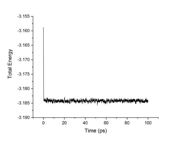
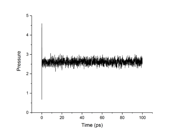
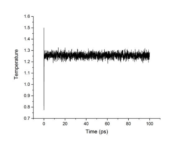
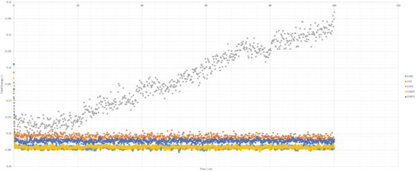
The largest timestep of 0.015 is a particularly bad choice as the energy does not converge, but increases dramatically, something which should not happen. The largest to give acceptable results is 0.0025, as though 0.001 and 0.0025 both converge to the same value, 0.0025 allows a simulation which simulates 250% more time than the 0.001 timestep. This is more practical as it allows more simulations and longer simulations to be done in the same time-frame as the smaller timestep, without losing accuracy or precision.tick

Running simulations under specific conditions

Temperature and Pressure Control

TASK: Choose 5 temperatures (above the critical temperature ), and two pressures (you can get a good idea of what a reasonable pressure is in Lennard-Jones units by looking at the average pressure of your simulations from the last section). This gives ten phase points — five temperatures at each pressure. Create 10 copies of npt.in, and modify each to run a simulation at one of your chosen  points. You should be able to use the results of the previous section to choose a timestep. Submit these ten jobs to the HPC portal. While you wait for them to finish, you should read the next section.

Thermostats and Barostats

TASK: We need to choose $\gamma$ so that the temperature is correct $T=\mathfrak{𝔗}$ if we multiply every velocity $\gamma$. We can write two equations:

$\frac{1}{2}\sum _i{m}_i{v}_i^2=\frac{3}{2}N{k}_{B}T$

$\frac{1}{2}\sum _i{m}_i{\left(\gamma v_i\right)}^2=\frac{3}{2}N{k}_B\mathfrak{𝔗}$

Solve these to determine $\gamma$.

$\frac{\frac{1}{2}\sum _i{m}_i{\left(\gamma v_i\right)}^2}{\frac{1}{2}\sum _i{v}_i^2}=\frac{\frac{3}{2}N{k}_B\mathfrak{𝔗}}{\frac{3}{2}N{k}_{B}T}$

$\frac{\sum _i{\left(\gamma v_i\right)}^2}{\sum _i{v}_i^2}=\frac{\mathfrak{𝔗}}{T}$

$\frac{\sum _i{\gamma }^2{v}_i^2}{\sum _i{v}_i^2}=\frac{\mathfrak{𝔗}}{T}$

$\frac{{\gamma }^2\sum _i{v}_i^2}{\sum _i{v}_i^2}=\frac{\mathfrak{𝔗}}{T}$

${\gamma }^2=\frac{\mathfrak{𝔗}}{T}$

$\gamma =\sqrt{\frac{\mathfrak{𝔗}}{T}}$

tick

Examining the Input Script

TASK: Use the manual page to find out the importance of the three numbers 100 1000 100000. How often will values of the temperature, etc., be sampled for the average? How many measurements contribute to the average? Looking to the following line, how much time will you simulate?

The first number defines the length of the timestep between data points taken for the calculation of the average, the second number relates to how many timesteps will be used to calculate the average at the specificed time, the last number specifies at what timestep will an average be taken. Thus 100 1000 100000 means that data points for the average will be taken every 100 timesteps, and 1000 will be used to calculate the average at 100000 timesteps. The time simulated will be 100000 * the timestep in seconds, which for 0.0025 s per timestep means that 250 s will be simulated.

TASK: When your simulations have finished, download the log files as before. At the end of the log file, LAMMPS will output the values and errors for the pressure, temperature, and density $\left(\frac{N}{V}\right)$. Use software of your choice to plot the density as a function of temperature for both of the pressures that you simulated. Your graph(s) should include error bars in both the x and y directions. You should also include a line corresponding to the density predicted by the ideal gas law at that pressure. Is your simulated density lower or higher? Justify this. Does the discrepancy increase or decrease with pressure?

A plot of average density against average critical temperature of the system with standard error error bars

The discrepancies between the idealised and simulated number density results can be attributed to the simulation being non-ideal. The basis of a L-J system is that the particles interact with each other, with a short range repulsive term, and a longer range attractive term. The ideal gas law however, assumes that there are no interactions between particles and thus, due to the short range highly repulsive term, the particles are further apart than in a system with no interactions and therefore the number density of the simulated systems are lower than their idealised counterparts.tick

At higher pressures the deviations from ideality are larger than that of a lower pressure simulation. This arises from the fact that at higher pressures, the number density is higher due to decreased cell volume, leading to decreased distances between particles and therefore increased interactions between them as they collide with each other more frequently. This increase in interactions between particles leads to a large deviation from ideality and so a larger difference between simulated and ideal law data for higher pressures.tick

Calculating heat capacities using statistical physics

Heat Capacity Calculation

TASK: As in the last section, you need to run simulations at ten phase points. In this section, we will be in density-temperature $({\rho }^{*},T^{*})$ phase space, rather than pressure-temperature phase space. The two densities required at $0.2$ and $0.8$, and the temperature range is $2.0,2.2,2.4,2.6,2.8$. Plot $C_V/V$ as a function of temperature, where $V$ is the volume of the simulation cell, for both of your densities (on the same graph). Is the trend the one you would expect? Attach an example of one of your input scripts to your report.

An image of one of the scripts used for the heat capacity calculations

A plot of $C_V/V$ against $T/T*$ for two different densities

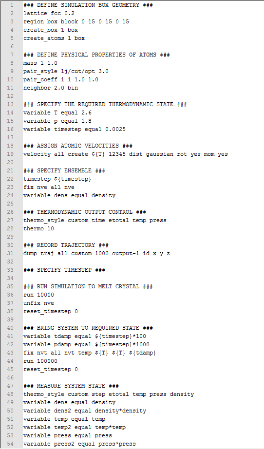
The decrease of heat capacity with temperature increase excluding phase changes, can be explained through the Density of States. Similar to the anharmonic oscillator model for electron excitation for an atom or particles where as the energy levels are increased, the spacing between the levels decrease, as the temperature of our system is increased the spacing between energy levels contracts, and thus the higher energy levels come down in energy and become more accessible. This leads to more modes available for promotion in the system, thus ease of promotion of an atom increases, leading to a reduced energy needed to promote and atom and so heat capacity decreases with temperature.tick

The large jumps in heat capacity seen in both data sets at $T^{*}=2.6$ can be explained through phase changes. As the particles simulated are totally symmetric there are no extra degrees of freedom to be reached through an increase in temperature as only translational modes are active through equipartition theorem, therefore the jump in heat capacity must be due to a phase change. Assuming a second order phase transition; as an NVT ensemble is used, and in a first order transition density is discontinuous which is impossible for a system with fixed $N$ and $V$, Heat capacity rises to infinity until after the transition has been completed, after which it lowers again, which can be seen at $T^{*}=2.8$, due to thermal energy needing to be expended in order to complete the phase transition.tick

Structural properties and the radial distribution function

Simulations in this section

TASK: perform simulations of the Lennard-Jones system in the three phases. When each is complete, download the trajectory and calculate $g(r)$ and $\int g(r)\mathrm{d}r$. Plot the RDFs for the three systems on the same axes, and attach a copy to your report. Discuss qualitatively the differences between the three RDFs, and what this tells you about the structure of the system in each phase. In the solid case, illustrate which lattice sites the first three peaks correspond to. What is the lattice spacing? What is the coordination number for each of the first three peaks?

Figure 4: ft1015G(r).png

Figure 4: ft1015G(r)N.png

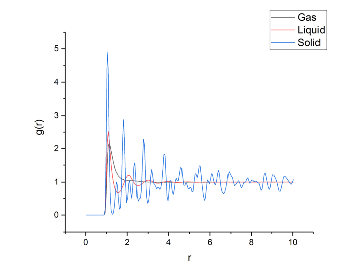
The RDF for the gas one broad peak that drops to 1 quickly after the peak finishes, leading to there being no long range order as the probability of finding an particle outside of the first shell is equal everywhere. This shows that there is no long range order in a gas, only extremely short range order. The peak could be broad due to weak attractive effects holding the nearest neighbors close, but not tightly holding them in place.tick

The liquid RDF has three broad peaks, leading to 3 co-ordination spheres of particles held tightly, but not so tightly that the particles cannot move, therefore the spheres are very lightly diffuse, but like the gas the RDF drops to 1 after the last peaking, leading to no long range order in a liquid.

The RDF of the solid has many sharp peaks corresponding to the solid atoms fixed positions and long range order in the crystal lattice.

The lattice spacing is the minimum distance between lattice unit cells which is equal to 1.175.tick

r	Integrated g(r)	Co-ordination Number
1.175	11.85813	12
1.675	18.44288	6
1.975	42.26256	24

Dynamical properties and the diffusion coefficient

Simulations in this Section

TASK: In the D subfolder, there is a file liq.in that will run a simulation at specified density and temperature to calculate the mean squared displacement and velocity autocorrelation function of your system. Run one of these simulations for a vapour, liquid, and solid. You have also been given some simulated data from much larger systems (approximately one million atoms). You will need these files later.

Mean Squared Displacement

TASK: make a plot for each of your simulations (solid, liquid, and gas), showing the mean squared displacement (the "total" MSD) as a function of timestep. Are these as you would expect? Estimate $D$ in each case. Be careful with the units! Repeat this procedure for the MSD data that you were given from the one million atom simulations.

From https://en.wikipedia.org/wiki/Mean_squared_displacementː

$MSD=⟨(x(t)-x_0{)}^2⟩=2Dt$

Figure 4: ft1015GasMSD.png

Figure 5: ft1015GasMSD_1m.png

Figure 6: ft1015LiquidMSD.png

Figure 7: ft1015LiquidMSD_1m.png

Figure 8: ft1015SolidMSD.png

Figure 9: ft1015SolidMSD_1m.png

EXTENSION: Velocity Autocorrelation Function

TASK: In the theoretical section at the beginning, the equation for the evolution of the position of a 1D harmonic oscillator as a function of time was given. Using this, evaluate the normalised velocity autocorrelation function for a 1D harmonic oscillator (it is analytic!):

$C\left(\tau \right)=\frac{\underset{-\mathrm{\infty }}{\overset{\mathrm{\infty }}{\int }}v\left(t\right)v(t+\tau )\mathrm{d}t}{\underset{-\mathrm{\infty }}{\overset{\mathrm{\infty }}{\int }}{v}^2\left(t\right)\mathrm{d}t}$

Be sure to show your working in your writeup. On the same graph, with x range 0 to 500, plot $C\left(\tau \right)$ with $\omega =1/2\pi$ and the VACFs from your liquid and solid simulations. What do the minima in the VACFs for the liquid and solid system represent? Discuss the origin of the differences between the liquid and solid VACFs. The harmonic oscillator VACF is very different to the Lennard Jones solid and liquid. Why is this? Attach a copy of your plot to your writeup.

TASK: Use the trapezium rule to approximate the integral under the velocity autocorrelation function for the solid, liquid, and gas, and use these values to estimate $D$ in each case. You should make a plot of the running integral in each case. Are they as you expect? Repeat this procedure for the VACF data that you were given from the one million atom simulations. What do you think is the largest source of error in your estimates of D from the VACF?

References

- ↑ Jean-Pierre Hansen and Loup Verlet, Phys. Rev. 184, 151
- ↑ Belén Zalba, José M Marı́n, Luisa F. Cabeza, Harald Mehling, Review on thermal energy storage with phase change: materials, heat transfer analysis and applications, In Applied Thermal Engineering, Volume 23, Issue 3, 2003, Pages 251-283
- ↑ Murat Kenisarin, Khamid Mahkamov, Solar energy storage using phase change materials, In Renewable and Sustainable Energy Reviews, Volume 11, Issue 9, 2007, Pages 1913-1965
- ↑ S. Mondal, Phase change materials for smart textiles – An overview, In Applied Thermal Engineering, Volume 28, Issues 11–12, 2008, Pages 1536-1550
- ↑ https://www.imperial.ac.uk/admin-services/ict/self-service/research-support/hpc/
- ↑ http://www.originlab.com/Origin
- ↑ http://cbio.bmt.tue.nl/pumma/index.php/Manual/ReducedUnits
- ↑ http://www.ks.uiuc.edu/Research/vmd/
- ↑ Phys. Chem. Chem. Phys.,2013, 15, 845