Overall feedback: The tasks were completed with quite a few mistakes. The report was very short and failed to convey a clear goal and motivation, but instead included vague statements about MD. Grammar and spelling were an issue. Please edit your work!.

Third year simulation experiment

Liquid simulation and the diffusion coefficient

Zhuohao You

Abstract

Diffusion behaviour of water was modeled and investigated by molecular dynamic simulation with the assistant of high performance computing power. The connection of diffusion coefficient to the mean square displacement was exploited to calculated the diffusion coefficient base on the performed MSD for liquid, solid and vapour. A further experiment on diffusion coefficient of solid was carried to exam its relationship with temperature. The abstract of a scientific paper is meant to briefly convey what you have done and your main results and conclusions, perhaps with a very short motivation. While you have briefly touched upon what you have done, your abstract lacks specifics. What exactly were your main results and conclusions? Also spelling and grammar!

Introduction

With the development of high performance computing system, the accuracy of molecular dynamic simulation (MSD) molecular dynamics is usually represented by the acronym "MD", "MDS" for molecular dynamics simulation(s) would be acceptable if specified. However "MSD" has the letters in the wrong order, and is a bit confusing given that MSD is also common for "mean squared displacement" was brought to a new level Arguably, yes. However, you have performed relatively small simulations using cheap and cheerful LJ potentials, so perhaps this comment is not very relevant to what you have done. . MSD is a useful tool that gives rise to calculation of macroscopic properties from microscopic scale systems. By considering the interaction for a single particle with a limited amount of nearby particles, 'exact' prediction of thermo and physical properties are possible depending in the scale of calculation. This point is arguable, since there a lot of technical subtleties, certainly an elaboration would be necessary after making such a bold claim with the use of "exact". [1]

Using the college's high performance computing facilities simply "the college's" is not an adequate accreditation of the hpc resources you have used. , simulation of simple liquid what about the other phases you have simulated? was performed and an important property of diffusion coefficient was computed from the simulation with a method manipulating its relationship with the mean squared displacement of ensemble particles.

Aims and Objectives

In this experiment, simulation using Lennard-Jones potential was applied on a simple liquid system. (e.g. Argon) why single out argon? have you used LJ parameters for argon? And investigation of the diffusion coefficient property of the system in liquid, solid and vapour phase was carried to give comparisons between the three states. Furtherly, a variation in temperature for the solid state was investigated to exploit the relationship between temperate and diffusion coefficient.

Methods

The input script was base on the given npt file with 8000 atoms and the molecular dynamic was calculated by the velocity Verlet algorithm with based on Lennard-Jones potential. All the simulation was completed on the college HPC system with the parallel computational pacakge LAMMPS. The diffusion coefficient was computed by the given method: The easiest way to measure $D$ is by exploiting its connection to the mean squared displacement.

$D = \frac{1}{6} \frac{\partial ⟨ r^{2} (t) ⟩}{\partial t}$

This is not sufficient information for another scientist to reproduce your results. What LJ parameters have you used, what cutoff? You mention the NPT ensemble, what pressure and temperature?

Results and discussion

The mean squared displacement (MSD), effectively measures how much the particles deviate from their equilibrium positions a more clear explanation would be valuable here . The value of MSD represents the extent of random motion in the system, and it can be calculated with the equation:

In this experiment, calculation of MSD was all completed by HPC and was given in the results.

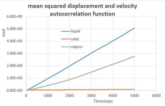
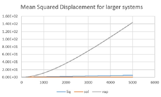
No x axis label for the second graph.

As shown in two graphs, the simulation for liquid, solid and vapour gives the evolution of mean squared displacement over ti,me for both cases. (8000 atoms and a million atoms respectively) The first thing to see on the graphs was the abnormal position for liquid state and gas state in the first figure, as the liquid phase gave a larger MSD as time goes, which on the other hand, for the second figure did have the gas curve laying above the liquid curve.

In a realistic sense, as the MSD measured the random of particles, the displacement for liquid molecules should be much smaller than the vapour counterpart, since the gas particles was supposed to be about 10 times more distant than liquid molecules in the space.

Therefore, it turn out that the simulation for vapour phase with this MSD method was inaccurate, or a much longer period of time was required for the system to reach the equilibrium.

As mentioned above, the diffusion coefficient was calculated by the relationship:

$D = \frac{1}{6} \frac{\partial ⟨ r^{2} (t) ⟩}{\partial t}$ so one sixth of the gradient of the MSD graph was the diffusion coeffient:

D(liq)= 0.000171 cm2/s; D(sol)= 1.92x10-6 cm2/s; D(vap)= 0.000106 cm2/s (8000atoms)

D(liq)= 0.000177cm2/s; D(sol)= 0; D(vap)= 0.00627cm2/s (a million atoms)

The result was quite close to each other apart from the vapour case, and the data confirmed that for the 8000 atoms system, an equilibrium was not reach therefore the inaccuracy was due to a lack of simulation steps as the gradient was only valid in the diffusion region of the graph (i.e. the linear part). In the case of solid the diffusion coefficient was to low to be calculated.

Extension

why have you included an extension in the middle of your results section? As the simulation for solid was quite stable in the last section, further interest of examine the temperate-diffusion coefficient connection was developed from the literature[2]. Five additional simulation with different temperature for the solid system was carried to investigate if the MDS simulation could give a similar trend.

T (reduced temperature)	Diffusion coefficient cm2/s
0.6	7.48E-07
0.7	7.85E-07
0.8	1.26E-06
0.9	1.47E-06
1.0	2.5E-06

The results of simulation was given in the table, and a clear trend of D increasing with temperature was illustrated.

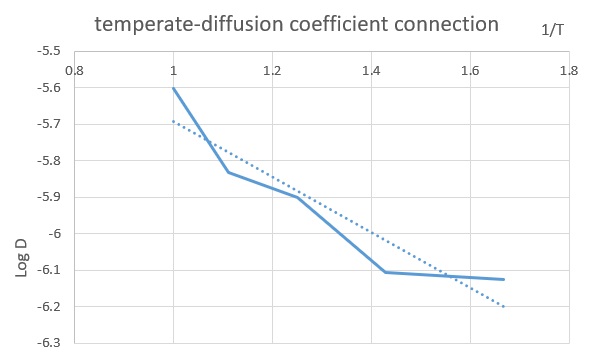
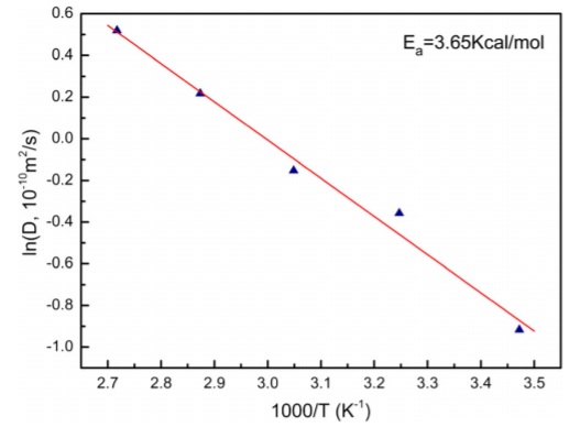
In general, the simulation gave the same relationship with the literature graph citation? , though the fluctuation in the computed curve was greater due to the weakness in size and timesteps. This was saying the error in the simulation can be averaged out with large scale simulation andFurther investigate of this relation could be carried with a greater size (e.g. a million atoms) and more steps to provide more reliable data for the different states.

Conclusion

The MD simulation provides a powerful and relatively reliable tool for investigation of the simple systems as shown in the experiment, this provides an alternative method to gather thermo and physical data from Lab experiment. To ensure the accuracy of the simulated data, a large size of model to mimic the interaction and long time of random motion to reach equillibrium was required.

These are some very vague conclusions. The conclusion of a scientific paper is meant to summarise the main results and conclusions, and perhaps offer a brief outlook.

Reference hav

Computational Soft Matter: From Synthetic Polymers to Proteins, Lecture Notes, Norbert Attig, Kurt Binder, Helmut Grubmuller ¨ , Kurt Kremer (Eds.), John von Neumann Institute for Computing, Julich, ¨ NIC Series, Vol. 23, ISBN 3-00-012641-4, pp. 1-28, 2004.
Molecular and condition parameters dependent diffusion coefficient of water in poly(vinyl alcohol): a molecular dynamics simulation study,Colloid and Polymer Science, 2017, 295(5),859-868

TASK:

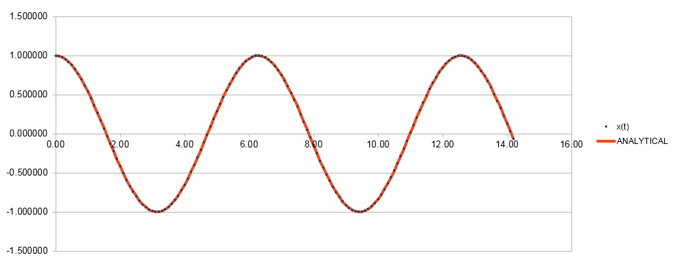
TASK: Open the file HO.xls. In it, the velocity-Verlet algorithm is used to model the behaviour of a classical harmonic oscillator. Complete the three columns "ANALYTICAL", "ERROR", and "ENERGY": "ANALYTICAL" should contain the value of the classical solution for the position at time , "ERROR" should contain the absolute difference between "ANALYTICAL" and the velocity-Verlet solution (i.e. ERROR should always be positive -- make sure you leave the half step rows blank!), and "ENERGY" should contain the total energy of the oscillator for the velocity-Verlet solution. Remember that the position of a classical harmonic oscillator is given by (the values of , , and are worked out for you in the sheet).

TASK: For the default timestep value, 0.1, estimate the positions of the maxima in the ERROR column as a function of time. Make a plot showing these values as a function of time, and fit an appropriate function to the data.

Error= C*t*sin( ωt + φ ) C is a constant that equals approx. 0.000417 in the case of timestep=0.1 ω=1.00 and φ=1.00

TASK: Experiment with different values of the timestep. What sort of a timestep do you need to use to ensure that the total energy does not change by more than 1% over the course of your "simulation"? Why do you think it is important to monitor the total energy of a physical system when modelling its behaviour numerically?

Timesteps below 0.63s would be valid in this case way too large . Ideally the total energy is conserved in a closed system, so it is better to monitor the total energy of a system to ensure the simulation was not collapsed in terms of a strong fluctuation in total energy.

force is +ve, r_eq is 2^(1/6)*sigma. Numerical answers stated to way too many decimal places.

TASK: Estimate the number of water molecules in 1ml of water under standard conditions. 55.5*N_A/1000= 3.34*10²²

Estimate the volume of 10000 water molecules under standard conditions. 10000/3.34*10²²=2.99*10^-19mL

Atom positions not after PBC not correct. Well depth off by factor of 1000, temperature not correct.

TASK: Why do you think giving atoms random starting coordinates causes problems in simulations? Hint: what happens if two atoms happen to be generated close together?

In case of two atoms generated on top of each other，the force between them will be very large and therefore leads to unwanted large acceleration to the system, cause a sudden blow up.

TASK: Satisfy yourself that this lattice spacing corresponds to a number density of lattice points of 0.8. Consider instead a face-centred cubic lattice with a lattice point number density of 1.2. What is the side length of the cubic unit cell? 1/(1.07722)3 = 0.800 4 atoms in one lattice, so 4/a3 = 1.2, a = 1.49380, side length is 1.49380.

TASK: Consider again the face-centred cubic lattice from the previous task. How many atoms would be created by the create_atoms command if you had defined that lattice instead? 4000

TASK: Using the LAMMPS manual, find the purpose of the following commands in the input script:

mass 1 1.0              for every atom in type 1 mass = 1.0 (reduced unit)
pair_style lj/cut 3.0   cutoff Lennard-Jones potential with no Coulomb at 3.0 potential with no Coulomb at 3.0
pair_coeff * * 1.0 1.0  for all the pairs coefficient 1.0 1.0 was applied

TASK: Given that we are specifying $x_{i} (0)$ and $v_{i} (0)$ , which integration algorithm are we going to use?

velocity Verlet algorithm.

TASK: Look at the lines below.

### SPECIFY TIMESTEP ###
variable timestep equal 0.001
variable n_steps equal floor(100/${timestep})
timestep ${timestep}

### RUN SIMULATION ###
run ${n_steps}
run 100000

The second line (starting "variable timestep...") tells LAMMPS that if it encounters the text ${timestep} on a subsequent line, it should replace it by the value given. In this case, the value ${timestep} is always replaced by 0.001. In light of this, what do you think the purpose of these lines is? Why not just write:

timestep 0.001
run 100000

Ask the demonstrator if you need help.

Allows easy variation of timesteps without worrying about forgetting to change the relevant steps to run. As the change in steps will be made by the codes as soon as the value of timesteps was changed. Instantaneous change of two related value.

TASK: make plots of the energy, temperature, and pressure, against time for the 0.001 timestep experiment (attach a picture to your report).

Does the simulation reach equilibrium? Yes

How long does this take? 0.3 reduced time

When you have done this, make a single plot which shows the energy versus time for all of the timesteps (again, attach a picture to your report).

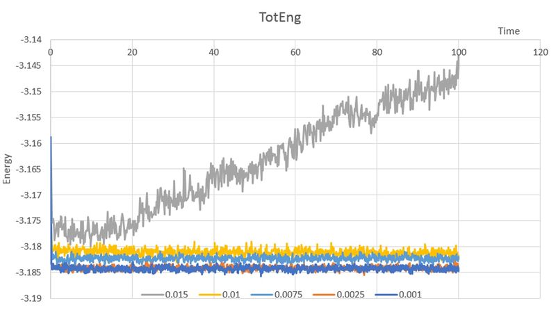
Choosing a timestep is a balancing act: the shorter the timestep, the more accurately the results of your simulation will reflect the physical reality; short timesteps, however, mean that the same number of simulation steps cover a shorter amount of actual time, and this is very unhelpful if the process you want to study requires observation over a long time. Of the five timesteps that you used, which is the largest to give acceptable results? 0.0025

Fluctuating in the region that covers the most accurate value from 0.0001

Which one of the five is a particularly bad choice? Why? 0.015 it does not converge.

TASK: We need to choose $γ$ so that the temperature is correct $T = 𝔗$ if we multiply every velocity $γ$ . We can write two equations:

$\frac{1}{2} \sum_{i} m_{i} v_{i}^{2} = \frac{3}{2} N k_{B} T$

$\frac{1}{2} \sum_{i} m_{i} {(γ v_{i})}^{2} = \frac{3}{2} N k_{B} 𝔗$

Solve these to determine $γ$ .

γ = ( $𝔗$ /T )0.5

I think you meant to the power of 0.5 here, but it is typed as multiply as 0.5. Be more careful! Also, if you showed any working out, then I could safely say this was a typo, but since you have not, I cannot justify treating it as to the power of 0.5

TASK: Use the manual page to find out the importance of the three numbers 100 1000 100000.

• Nevery = 100 use input values every 100 timesteps

• Nrepeat = 1000 1000 of times to use input values for calculating averages

• Nfreq =10000 calculate averages every 10000 timesteps

How often will values of the temperature, etc., be sampled for the average? every 10000 timesteps

How many measurements contribute to the average? 1000

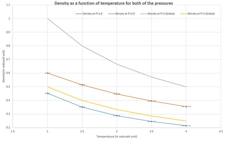
Looking to the following line, how much time will you simulate? 100000 unit time TASK: When your simulations have finished, download the log files as before. At the end of the log file, LAMMPS will output the values and errors for the pressure, temperature, and density $(\frac{N}{V})$ . Use software of your choice to plot the density as a function of temperature for both of the pressures that you simulated.

Your graph(s) should include error bars in both the x and y directions. You should also include a line corresponding to the density predicted by the ideal gas law at that pressure. Is your simulated density lower or higher? Justify this. Does the discrepancy increase or decrease with pressure?

Lower, as ideal gas law ignores any interactions between particles apart from collisions while the L-J system takes the potential energy into account so that results in a lower density. discrepancy increase with pressure.

TASK: As in the last section, you need to run simulations at ten phase points. In this section, we will be in density-temperature $(ρ^{*}, T^{*})$ phase space, rather than pressure-temperature phase space. The two densities required at $0.2$ and $0.8$ , and the temperature range is $2.0, 2.2, 2.4, 2.6, 2.8$ . Plot $C_{V} / V$ as a function of temperature, where $V$ is the volume of the simulation cell, for both of your densities (on the same graph). Is the trend the one you would expect? Attach an example of one of your input scripts to your report.

Supposed to be constant for liquid but the fluctuation was within an acceptable range

Scripts:

### SPECIFY THE REQUIRED THERMODYNAMIC STATE ###

variable D equal 0.2

variable T equal 2.0

variable timestep equal 0.0025

### DEFINE SIMULATION BOX GEOMETRY ###

lattice sc ${D}

region box block 0 15 0 15 0 15

create_box 1 box

create_atoms 1 box

### DEFINE PHYSICAL PROPERTIES OF ATOMS ###

mass 1 1.0

pair_style lj/cut/opt 3.0

pair_coeff 1 1 1.0 1.0

neighbor 2.0 bin

### ASSIGN ATOMIC VELOCITIES ###

velocity all create ${T} 12345 dist gaussian rot yes mom yes

### SPECIFY ENSEMBLE ###

timestep ${timestep}

fix nve all nve

### THERMODYNAMIC OUTPUT CONTROL ###

thermo_style custom time etotal temp press

thermo 10

### RECORD TRAJECTORY ###

dump traj all custom 1000 output-1 id x y z

### RUN SIMULATION TO MELT CRYSTAL ###

run 10000

unfix nve

reset_timestep 0

### BRING SYSTEM TO REQUIRED STATE ###

variable tdamp equal ${timestep}*100

variable pdamp equal ${timestep}*1000

fix nvt all nvt temp ${T} ${T} ${tdamp}

run 10000

reset_timestep 0

unfix nvt

fix nve all nve

### MEASURE SYSTEM STATE ###

thermo_style custom step etotal temp vol density

variable dens equal density

variable temp equal temp

variable volu equal vol

variable ener equal etotal

variable ener2 equal etotal*etotal

fix aves all ave/time 100 1000 100000 v_dens v_temp v_vol v_ener v_ener2 v_press2

run 100000

variable avedens equal f_aves[1]

variable avetemp equal f_aves[2]

variable avevolu equal f_aves[3]

variable heatc equal 3375*3375*(f_aves[5]-f_aves[4]*f_aves[4])/(f_aves[2]*f_aves[2])

print "Averages"

print "--------"

print "Density: ${avedens}"

print "Volume: ${avevolu}"

print "Temperature: ${avetemp}"

print "Cv/V: ${heatc}/${avevolu}"

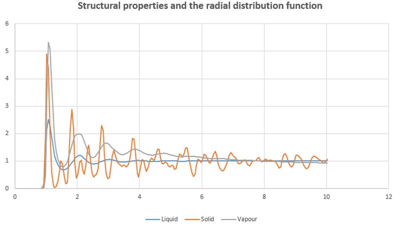
TASK: perform simulations of the Lennard-Jones system in the three phases. When each is complete, download the trajectory and calculate $g (r)$ and $\int g (r) d r$ . Plot the RDFs for the three systems on the same axes, and attach a copy to your report.

Discuss qualitatively the differences between the three RDFs, and what this tells you about the structure of the system in each phase.

Liquid and vapour drop constantly due to the evenly distributing simple cubic structure while solid has fluctuation because of the Fcc structure.

This does not really make sense, are you saying that the gas and liquid phase form a cubic lattice? - Then they would be the solid phase! We were looking for a discussion of the short range vs. long range order for each of the phases, relating this to the features of the RDF.

In the solid case, illustrate which lattice sites the first three peaks correspond to. What is the lattice spacing?

What is the coordination number for each of the first three peaks?

Lattice spacing around 1.45 reduced unit.

[0.5,0.5,0] corners; [1.0,0,0] centre of face; [1.0,0.5,0] centre of a different face

Illustration? What are the coordination numbers?

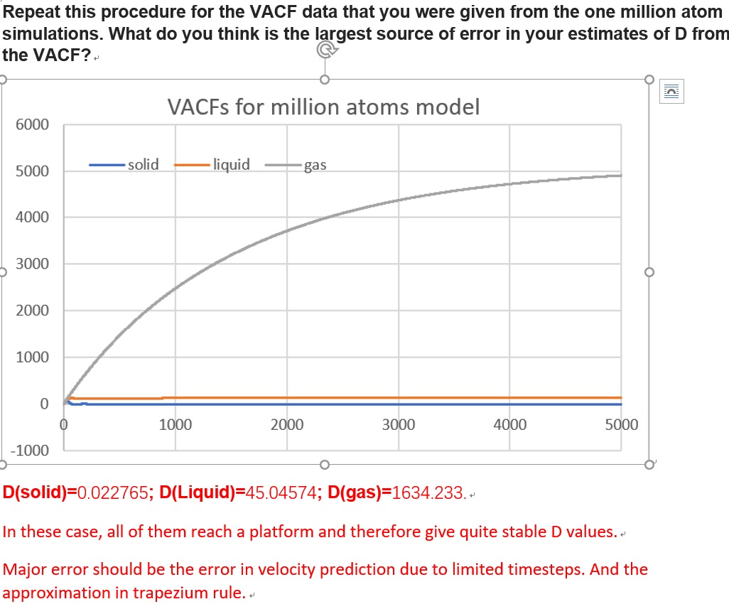
TASK: make a plot for each of your simulations (solid, liquid, and gas), showing the mean squared displacement (the "total" MSD) as a function of timestep. Are these as you would expect? Estimate in each case. Be careful with the units! Repeat this procedure for the MSD data that you were given from the one million atom simulations.

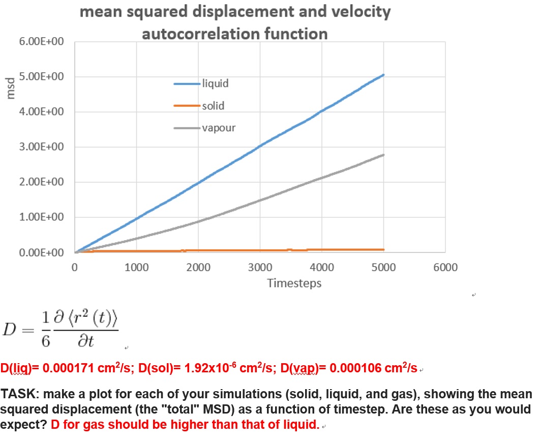
Yes diffusion coefficient should be higher for the gas than liquid - this data is not so good.

TASK: In the theoretical section at the beginning, the equation for the evolution of the position of a 1D harmonic oscillator as a function of time was given. Using this, evaluate the normalised velocity autocorrelation function for a 1D harmonic oscillator (it is analytic!):

$C (τ) = \frac{\int_{- \infty}^{\infty} v (t) v (t + τ) d t}{\int_{- \infty}^{\infty} v^{2} (t) d t}$

Be sure to show your working in your writeup.

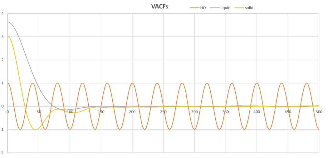
On the same graph, with x range 0 to 500, plot $C (τ)$ with $ω = 1 / 2 π$ and the VACFs from your liquid and solid simulations. What do the minima in the VACFs for the liquid and solid system represent?

The minima give the location of the maximum difference for the liquid and solid system.

This is not what we were looking for. Think about was the VACF actually corresponds to, and how the velocity changes after initiating the simulation. What happens when they particles begin to collide?

Discuss the origin of the differences between the liquid and solid VACFs. The harmonic oscillator VACF is very different to the Lennard Jones solid and liquid. Why is this?

Because the HO model has a periodic motion while the Lennard Jones solid and liquid move randomly there for there is no pattern in this kind of motion. i.e. the dependence on previous velocity is rather low. Could be better explained - I get what you are trying to say. First of all LJ particles do not move randomly... or what would be the point of the simulation? But unlike the LJ system, the velocity of a simple HO in a closed system is exactly periodic.

Attach a copy of your plot to your writeup.