Rep:Y3C Liquid Simulation:hjt14

Section 1: Running First Simulation

No task.

Section 2: Introduction to Molecular Dynamics Simulation

Numerical Integration

Task

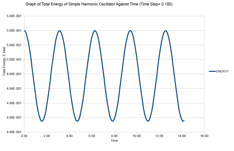
Link to the completed HO.xls file. The followings are the graph constructed using data from the excel worksheet. The first graph is an overlap of two graph of position of simple harmonic oscillator, $x(t)$, as a function of time, $t$; one calculated using velocity verlet algorithm, and one calculated using $x\left(t\right)=A\cos (\omega t+\varphi )$. The second graph is the graph of total energy of the simple harmonic oscillator, $E_{total}(t)$, as a function of time, $t$. The third graph is the graph of absolute error (difference between in position, $x(t)$, calculated using classical harmonic oscillator solution and calculated using velocity verlet algorithm) as a function of time, $t$. The maximas were located from each parabola and were fitted with a linear function. The equation of the linear function is displayed on the graph.

Graphs from excel file
Graph 1
Graph 2
Graph 3

Since we are working in a close system, i.e., no energy exchange with surrounding, the total energy of the system should be a constant. What we observed from graph 2 is that the total energy of the system oscillates about an average value. The deviation from the average energy is treated as the error introduced by the approximation we made in velocity verlet algorithm. The percentage error of total energy at different timestep were computed using following equation and the results are summarized in graph 4:

Percentage Error $=\frac{(E_{max}-E_{min})}{2\times E_{average}}\times 100\mathrm{\%}$

Graph 4

It can be seen from graph 4 that for timestep beyond 0.28, the percentage error in total energy will exceed 1%.

Atomic Forces

Task

Lennard-Jones Equation: $\varphi (r)=4ϵ(\frac{{\sigma }^{12}}{r^{12}}-\frac{{\sigma }^6}{r^6})$

When potential energy is set to zero, i.e.$\varphi =0$:

$0=4ϵ(\frac{{\sigma }^{12}}{r^{12}}-\frac{{\sigma }^6}{r^6})$

$\frac{{\sigma }^{12}}{r^{12}}=\frac{{\sigma }^6}{r^6}$

$\frac{{\sigma }^6}{r^6}=1$

$\sigma =r=r_0$

The value of $r$ when potential energy $\varphi$ is set to zero,$r_0$, is equal to $\sigma$.

The force acting on a particle a distance $r$ away from another particle can be calculated using following equation:

$F=-\frac{d\varphi (r)}{dr}$

$F=4ϵ(\frac{12{\sigma }^{12}}{r^{13}}-\frac{6{\sigma }^6}{r^7})$

When $r=r_0=\sigma$:

$F=4ϵ(\frac{12{\sigma }^{12}}{{\sigma }^{13}}-\frac{6{\sigma }^6}{{\sigma }^7})$

$F=4ϵ(\frac{12}{\sigma }-\frac{6}{\sigma })$

$F=\frac{24ϵ}{\sigma }$

At distance $r_0$, where the potential energy, $\varphi$, is zero, the force acting on a particle is equal to $\frac{24ϵ}{\sigma }$.

When $F=0$, defines $r=r_{eq}$:

$F=0=4ϵ(\frac{12{\sigma }^{12}}{r_{eq}^{13}}-\frac{6{\sigma }^6}{r_{eq}^7})$

$\frac{12{\sigma }^{12}}{r_{eq}^{13}}=\frac{6{\sigma }^6}{r_{eq}^7}$

$2{\sigma }^6=r_{eq}^6$

$r_{eq}=\sqrt[6]{2}\sigma$

The equilibrium distance,$r_{eq}$ , between 2 particles, which is defined as separation of 2 particles when the force acting on each particle is zero, is equal to $\sqrt[6]{2}\sigma$, $\sigma$ is a constant and is specific to particle under study. At equalibrium distance, $r_{eq}$, the potential energy, $\varphi (r_{eq})$, is at minimum and can be caculated as follow:

$\varphi (r_{eq})=4ϵ(\frac{{\sigma }^{12}}{(\sqrt[6]{2}\sigma {)}^{12}}-\frac{{\sigma }^6}{(\sqrt[6]{2}\sigma {)}^6})$

$\varphi (r_{eq})=4ϵ(\frac{1}{4}-\frac{1}{2})$

$\varphi (r_{eq})=-ϵ$

The following part shows the working of the integration of potential energy, $\varphi$, with respect to $r$. The integral is equivalent to the area under the potential energy graph encompassed by the integration range, $x$ to $y$.

$\underset{x}{\overset{y}{\int }}\varphi (r)dr=\underset{x}{\overset{y}{\int }}4ϵ(\frac{{\sigma }^{12}}{r^{12}}-\frac{{\sigma }^6}{r^6})dr$

$\underset{x}{\overset{y}{\int }}\varphi (r)dr=4ϵ{[\frac{-{\sigma }^{12}}{11r^{11}}+\frac{{\sigma }^6}{5r^5}]}_x^y$

When $ϵ=1$ and $\sigma =1$:

$\underset{x}{\overset{y}{\int }}\varphi (r)dr=4{[\frac{-1^{12}}{11r^{11}}+\frac{1^6}{5r^5}]}_x^y$

When $x=2\sigma =2$ and $y=\mathrm{\infty }$:	When $x=2.5\sigma =2.5$ and $y=\mathrm{\infty }$:	When $x=3\sigma =3$ and $y=\mathrm{\infty }$:
$\underset{2}{\overset{\mathrm{\infty }}{\int }}\varphi (r)dr=4{[\frac{-1^{12}}{11r^{11}}+\frac{1^6}{5r^5}]}_2^{\mathrm{\infty }}$ $\underset{2}{\overset{\mathrm{\infty }}{\int }}\varphi (r)dr=4[0-(\frac{-1^{12}}{11(2^{11})}+\frac{1^6}{5(2^5)})]$ $\underset{2}{\overset{\mathrm{\infty }}{\int }}\varphi (r)dr=-\frac{699}{28160}=-0.0248$	$\underset{2.5}{\overset{\mathrm{\infty }}{\int }}\varphi (r)dr=4{[\frac{-1^{12}}{11r^{11}}+\frac{1^6}{5r^5}]}_{2.5}^{\mathrm{\infty }}$ $\underset{2.5}{\overset{\mathrm{\infty }}{\int }}\varphi (r)dr=4[0-(\frac{-1^{12}}{11(2.5^{11})}+\frac{1^6}{5(2.5^5)})]$ $\underset{2.5}{\overset{\mathrm{\infty }}{\int }}\varphi (r)dr=-0.00818$	$\underset{3}{\overset{\mathrm{\infty }}{\int }}\varphi (r)dr=4{[\frac{-1^{12}}{11r^{11}}+\frac{1^6}{5r^5}]}_3^{\mathrm{\infty }}$ $\underset{3}{\overset{\mathrm{\infty }}{\int }}\varphi (r)dr=4[0-(\frac{-1^{12}}{11(3^{11})}+\frac{1^6}{5(3^5)})]$ $\underset{3}{\overset{\mathrm{\infty }}{\int }}\varphi (r)dr=-0.00329$

Periodic Boundary Conditions

Task

The number of water molecules in 1 ml of water under standard conditions (298K and 1 atm) is calculated as follow:

Density of water under standard conditions$=0.9970gm{l}^{-1}$

Mass of 1 ml of water $=0.9970g$

Molar mass of water $=2(1.008)+15.999=18.015gmo{l}^{-1}$

Number of water molecule in 1 ml of water $=\frac{0.9970(6.022\times 10^{23})}{18.015}=3.333\times 10^{22}$

The volume occupied by 1000 water molecules under standard conditions is calculated as follow:

Mass of 1000 water molecules $=\frac{1000}{6.022\times 10^{23}}(18.015)=2.992\times 10^{-20}g$

Volume occupied by 1000 water molecules $=\frac{2.992\times 10^{-20}}{0.9970}=3.001\times 10^{-20}ml$

Task

Under periodic boundary condition, the final position of an atom, after it move from $\left(\begin{array}{c}0.5\\ 0.5\\ 0.5\end{array}\right)$ by $\left(\begin{array}{c}0.7\\ 0.6\\ 0.2\end{array}\right)$ in a cubic simulation box which runs from $(0,0,0)$ to $(1,1,1)$, can be calculated as follow:

New position of atom $=\left(\begin{array}{c}0.5\\ 0.5\\ 0.5\end{array}\right)+\left(\begin{array}{c}0.7\\ 0.6\\ 0.2\end{array}\right)=\left(\begin{array}{c}1.2\\ 1.1\\ 0.7\end{array}\right)$

Apply periodic boundary condition:

New position of atom $=\left(\begin{array}{c}1.2-1\\ 1.1-1\\ 0.2\end{array}\right)=\left(\begin{array}{c}0.2\\ 0.1\\ 0.2\end{array}\right)$

Reduced Units

Task

The real units, $r$, is calculated as follow:	The well depth in $kJmo{l}^{-1}$ is calculated as follow:	The reduced temperature $T^{*}=1.5$ in real units is calculated as follow:
$r^{*}=\frac{r}{\sigma }$ $r^{*}=3.2$ and $\sigma =0.34nm$ $r=3.2(0.34)nm$ $r=1.088nm$	$\frac{ϵ}{N_A{k}_B}=120K$ $\frac{ϵ}{R}=120K$ $ϵ=120(8.31)Jmo{l}^{-1}$ $ϵ=997Jmo{l}^{-1}=0.997kJmo{l}^{-1}$	$T^{*}=\frac{k_{B}T}{ϵ}$ $1.5=\frac{1}{120}T$ $T=180K$

Section 3: Equilibration

Creating the Simulation Box

Task

Within an input file for molecular simulation, the initial conditions stipulated may not be the equilibrium conditions. During a simulation, LAMMPS will try to bring the system down to the equilibrium state by iteration within the allowed timesteps specified in the input file. If random coordinate is assigned to each atom, there is a chance that two or more atoms will be assigned coordinates that are too close together. This will mean that the atoms overlap in space. According to Lennard-Jones equation, this condition will give rise to the extremely high potential energy (approach infinity) and large repulsion between atoms. As a result of this situation, calculations done using LAMMPS sumulator will run into errors and the system will not be brought to equilibrium state.

Task

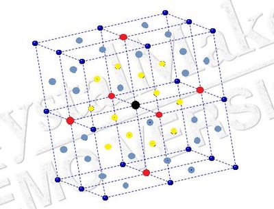
A unit cell of a simple cubic lattice is a cube dotted with lattice point at each vertice. Each vertice is shared between 4 unit cells, hence each vertice will contribute a quarter of a lattice point to a unit cell. Consequently, each unit cell will have lattice point, 4 corners each contributes a quarter of a lattice point. The number density can be calculated by dividing the number of lattice point in a unit cell by the volume of a unit cell.

If we have a unit cell of size $1.07722\times 1.07722\times 1.07722$ (in redued units):

Number density of a simple cubic lattice $=\frac{1}{1.07722\times 1.07722\times 1.07722}=0.8$

If we have a face-centered cubic lattice with lattice point number density of $1.2$, we can calculate the size of unit cell as follow:

Number of lattice point in a face-centered cubic unit cell $=4$

Volume of unit cell $=l\times l\times l=l^3$

$l^3=\frac{4}{1.2}=3\frac{1}{3}$

$l=\sqrt[3]{3\frac{1}{3}}=1.49$

The lattice parameter of a face-centered cubic lattice with lattice point number density of $1.2$ is $1.49$ (in reduced units).

Task

The number of unit cell created in the defined region is $1000$. In each face-centered cubic unit cell, $4$ atoms will be generated. Consequently, the total number of atom that will be generated if a face-centered cubic lattice is used instead of a simple cubic lattice is $4000$.

Setting the Properties of the Atoms

Task

mass 1 1.0 pair_style lj/cut 3.0 pair_coeff * * 1.0 1.0

The first line of the command set the mass of the atom of type 1 to 1.0 (reduced units). The second line of the command defines the equation used to model the pairwise interaction energy between atoms. In this example, we are using Lennard-Jones Equation with a cutoff distance of 3.0 (reduced units). The third line of the command defines the coefficients of Lennard-Jones Equation, i.e $ϵ=\sigma =1.0$. The asterisks (* *) mean that the Lennard-Jones model will be imposed on every pair of atoms.

Task

Given that we are specifying $x_i\left(0\right)$ and $v_i\left(0\right)$, the integration algorithm that we will be using is velocity verlet algorithm.

Running the Simulation

Task

### SPECIFY TIMESTEP ###
variable timestep equal 0.001
variable n_steps equal floor(100/${timestep})
variable n_steps equal floor(100/0.001)
timestep ${timestep}
timestep 0.001

### RUN SIMULATION ###
run ${n_steps}
run 100000

By assigning a variable (timestep) to timestep (the value), it allows us to call 'timestep' at other part of the input script, meaning that we do not have to retype the exact value of timestep repeatly and allow us to call it simply by typing ${timestep}. Another advantage of assigning a variable (timestep) to timestep (the value), is that if we need to change the timestep of a simulation, we only need to change the value assigned to the variable 'timestep' and timestep in other part of the input file will be updated accordingly.

Checking Equilibrium

Task

Graphs Obtained at 0.001 Timestep

Graph 5

Graph 6

Graph 7

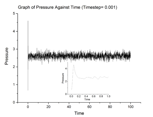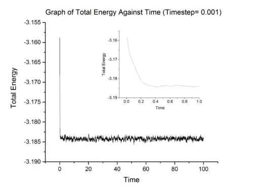
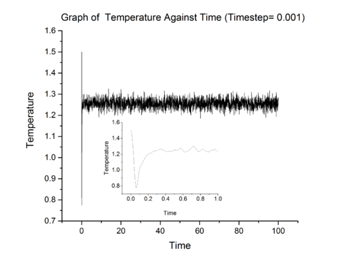
Above show three graphs obtained from LAMMPS simulation ran at 0.001 timestep. It can be seen that the system did achieved equilibrium and the inset in each graph show that system achieve equilibrium in approximately 0.4 fs. LAMMPS simulations were also ran at other timestep and the results for total energy were summarised in graph 8.

Graph 8

From graph 8, it can be seen that the most suitable timestep is 0.0025 as it is the maximum value which still allow the system under study to achieve equilibrium (a compromise between accuracy and time). 0.015 is a particularly bad choice because the system simulated at that timestep did not converge.

Section 4: Running Simulations under Specific Conditions

Thermostats and Barostats

Task

In order to bring the system to target temperature, $\mathfrak{𝔗}$, we multiply the velocity of each particle with a constant factor, $\gamma$, which will help to modulate the velocity of each atoms. The factor,$\gamma$, can be derived as follow:

$E_K=\frac{1}{2}\sum _i{m}_i{v}_i^2=\frac{3}{2}N{K}_{B}T$

Let $T=\mathfrak{𝔗}$ and multiply velocity of each atom with a constant factor, $\gamma$

$E_K=\frac{1}{2}\sum _i{m}_i{\gamma }^2{v}_i^2=\frac{3}{2}N{K}_B\mathfrak{𝔗}$

${\gamma }^2\frac{1}{2}\sum _i{m}_i{v}_i^2=\frac{3}{2}N{K}_B\mathfrak{𝔗}$

${\gamma }^2\frac{3}{2}N{K}_{B}T=\frac{3}{2}N{K}_B\mathfrak{𝔗}$

$\gamma =\sqrt{\frac{\mathfrak{𝔗}}{T}}$

Examining the Input Script

Task

fix aves all ave/time 100 1000 100000 v_dens v_temp v_press v_dens2 v_temp2 v_press2

The numbers and its position in the series will affect how the averages are calculated. The roles that each number play are summarised as follow:

Position	Value	Role
First	100	Sample data every 100 timestep
Second	1000	Perform sampling 1000 times
Third	100000	Average all the sampled data collected within 100000 timestep

Plotting the Equations of State

Task

Conditions used		Graph
Pressure	Temperature
2.0	1.8	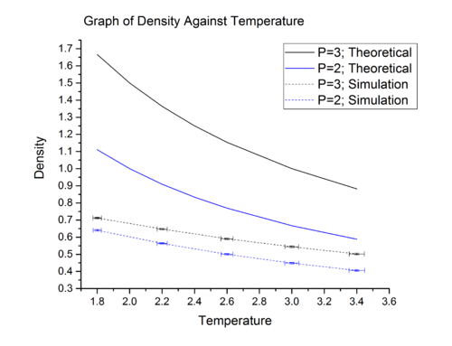Graph 9
	2.0
	2.2
	2.4
	2.6
3.0	1.8
	2.0
	2.2
	2.4
	2.6

Shown in the table, are 10 phase points used in LAMMPS molecular dynamic simulation to compute density under these conditions. The theoretical value of density at these phase points were also calculated using reduced ideal gas equation. The simulated density and calculated density are summarised in graph 9. The reduced ideal gas equation used in calculation is shown below:

$\rho =\frac{P}{T^{*}};\rho =\frac{N}{V}$

In graph 9, it can be seen that:

a) at all temperature, the simulated density are lower than the theoretical density.

Explanation: In ideal gas, we assume there are no inter-molecular interactions between particles, i.e., no attraction and no repulsion. However, in our LAMMPS simulation, we model the inter-molecular interactions using Lennord-Jones equation and this breaks the fundamental assumption made in the derivation of ideal gas equation. According to Lennard-Jones equation, below a certain bond distance, a particles pair will experience repulsive forces which will keep them at a distance away from each other. In this case, the particles are further apart from each other than they would be if they behave ideally. Consequently, the number of particle per unit volume, which is the density, is lowered.

b) the simulated density deviate considerably from ideal behavior at low temperature. At higher temperature, the magnitude of deviation decreases and the theoretical density and simulated density start to converge to a single value.

Explanation: At low temperature, the thermal energy, $k_{B}T$, is small relative to the interaction energy. Therefore the interaction energy can not be neglected and contribute significantly to the thermodynamic properties of our system. As temperature starts to increase, the thermal energy increases and at one point the magnitude of the thermal energy will become comparable to the interaction energy. At that point, the interactions between particles can be easily perturbed by thermal fluctuation and hence become irrelevant in determining the thermodynamic properties of our system. In other words, at higher temperature, interactions between particles become insignificant and system approaches ideal behavior. Therefore, simulated density and theoretical density converge to a single value.

Section 5: Calculating Heat Capacities Using Statistical Physics

Task

Link to one of the input file.

Conditions used		Graph
Density	Temperature
0.2	2.0	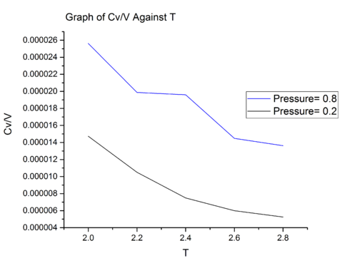Graph 10
	2.2
	2.4
	2.6
	2.8
0.8	2.0
	2.2
	2.4
	2.6
	2.8

Pressure is defined as $\frac{N}{V}$, at higher pressure there will be more particle per unit volume. In section 4, we encounter following equation which correlates the instantaneous temperature of a system to total kinetic energy:

$E_K=\frac{3}{2}N{k}_{B}T=\frac{1}{2}\sum _i{m}_i{v}_i^2$

Occupying the same volume, a system at higher pressure will have a greater number of particles. Therefore, for the same increment in temperature, the energy we need to provide to a system at higher density is greater than that of a system at lower pressure simply because there are more particles to which we have to provide the energy. Consequently, the heat capacity per unit volume of a system at higher pressure is greater than that of system at lower pressure simply because we need to provide more energy for the same increment in temperature.

According to equipartition theorem, each degree of freedom of an atom will contribute $\frac{1}{2}{k}_B$ to the total heat capacity of the system. As we are modeling a constant number of atoms, we expect the heat capacity of the system to be a constant. For both graphs, there is no clear reason to why the heat capacity reduces with temperature. One possible reason is that the density of state decreases with temperature. Higher density of state means that the energy levels are closer together and are easy to populate the energy states and hence correlate to lower heat capacity; Lower density of state means that the energy gap between energy levels is larger and and are difficult to populate the energy states. For same increment in temperature, greater energy need to be provided, and hence this correlate to higher heat capacity. One way to verify this is to obtain a plot of density of state versus energy.

Section 6: Structural Properties and the Radial Distribution Function

Calculating $g(r)$ in VMD

Task

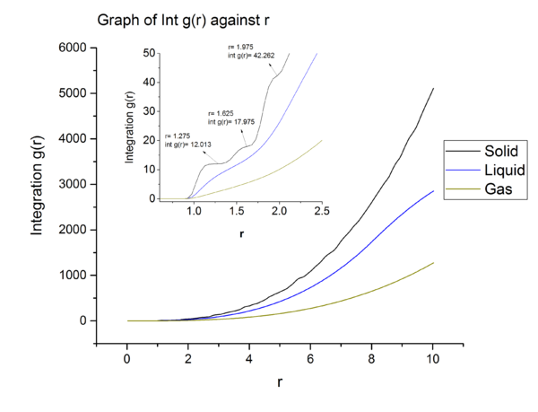
$g(r)$ can be understood as the number of particle per unit volume of shell of size $dr$ divided by the bulk density.

Graphs	Observed trends in graphs when going from solid to liquid and to gas	Remark
Graph 11 Graph 12	The peak intensity decreases and has greater width	In solid, the atoms are closely packed and hence are in higher coordination environment and this translates into high $g(r)$. From solid to gas, the coordination environment drop as the atoms are more loosely packed in this case and hence $g(r)$ decreases from solid to gas. The width of the peak is related to the distribution of $r$of atoms in the first coordination shell, then second coordination shell and etc.. In solid, the peaks are more confined than that of liquid and gas. This is because solid has low degree of freedom in motion, i.e., no translation, hence $r$ of atoms in each coordination shell has smaller distribution and this gives rise to relatively sharp peaks. From liquid to gas, the translational degree of freedom increases, and hence the position of atoms in coordination shell becomes less and less well defined. This uncertainty in $r$gives rise to wide peaks.
	The rate of decay of $g(r)$ increases	This is because solid has long range order in the spatial arrangement of atoms. In liquid and gas, the ordered structure is short range and over $r$ the peaks flattened out as atoms distribution is getting more and more random.
	Coordination environment decreases	REFERRING TO SOLID The first coordination shell of solid consisted of 12 particles (cuboctahedron) and corresponds to the first peak of solid $g(r)$ plot. The second coordination shell of solid consists of 6 particles (octahedron) and corresponds to the second peak of solid $g(r)$ plot. The third coordination shell of solid consists of 24 particles and corresponds to the third peak of solid $g(r)$ plot. The position of atoms in these shells are shown below relative to a reference point (coloured black): FCC lattice made using crystal maker. Black atom is the reference atom, yellow atoms are in the first coordination shell, red atoms are in the second coordination shell and grey atoms are in the third coordination shell. The lattice spacing of FCC lattice of solid is the same as the radius of the second coordination shell and is equal to 1.475 (refer graph 11)

Section 7: Dynamic Properties and the Diffusion Coefficient

Mean Squared Displacement

Task

Graph 13

Graph 14

State Gradient (w.r.t. time) Diffusion Coefficient (w.r.t. time) Gas (million) 18.19 (linear part) 3.032 Gas 4.915 0.8192 Liquid (million) 0.5236 0.08727 Liquid 0.5094 0.0849 Solid (million) 0.00002635 0.000004392 Solid 0.00535 0.000892

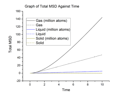
From graph 13, it can be seen that the diffusion coefficients increase from solid to gas and these are expected. In solid, the particles are closely packed, to diffuse, solid particles have to overcome large repulsion when sliding pass other particles and this contribute to the large activation energy for diffusive motion. Hence solid has negligible diffusion coefficient due to large energy barrier. From liquid to gas, the packing decreases meaning that the particles are further apart, making it easier for particle to move pass each other. The is reflected in the increase in diffusion coefficient when going from liquid to gas.

Velocity Autocorrelation Function

Task

$x(t)=A\cos (\omega t+\varphi );v(t)=\frac{dx(t)}{dt}=-A\omega \sin (\omega t+\varphi )$

$C\left(\tau \right)=\frac{\underset{-\mathrm{\infty }}{\overset{\mathrm{\infty }}{\int }}v\left(t\right)v(t+\tau )\mathrm{d}t}{\underset{-\mathrm{\infty }}{\overset{\mathrm{\infty }}{\int }}{v}^2\left(t\right)\mathrm{d}t}$

$C\left(\tau \right)=\frac{\underset{-\mathrm{\infty }}{\overset{\mathrm{\infty }}{\int }}{A}^2{\omega }^2\sin (\omega t+\varphi )\sin (\omega t+\omega \tau +\varphi )\mathrm{d}t}{\underset{-\mathrm{\infty }}{\overset{\mathrm{\infty }}{\int }}{A}^2{\omega }^2{\sin }^2(\omega t+\varphi )\mathrm{d}t}$

$C\left(\tau \right)=\frac{\underset{-\mathrm{\infty }}{\overset{\mathrm{\infty }}{\int }}{A}^2{\omega }^2\sin (\omega t+\varphi )(\sin (\omega t+\varphi )\cos \omega \tau +\cos (\omega t+\varphi )\sin \omega \tau )\mathrm{d}t}{\underset{-\mathrm{\infty }}{\overset{\mathrm{\infty }}{\int }}\frac{A^2{\omega }^2}{2}(1-\cos (2\omega t+2\varphi ))\mathrm{d}t}$

$C\left(\tau \right)=\frac{A^2{\omega }^2\underset{-\mathrm{\infty }}{\overset{\mathrm{\infty }}{\int }}{\sin }^2(\omega t+\varphi )\cos \omega \tau +\sin (\omega t+\varphi )\cos (\omega t+\varphi )\sin \omega \tau \mathrm{d}t}{\frac{A^2{\omega }^2}{2}\underset{-\mathrm{\infty }}{\overset{\mathrm{\infty }}{\int }}(1-\cos (2\omega t+2\varphi ))\mathrm{d}t}$

$C\left(\tau \right)=\frac{\underset{-\mathrm{\infty }}{\overset{\mathrm{\infty }}{\int }}(1-\cos (2\omega t+2\varphi ))\cos \omega \tau +2\sin (\omega t+\varphi )\cos (\omega t+\varphi )\sin \omega \tau \mathrm{d}t}{\underset{-\mathrm{\infty }}{\overset{\mathrm{\infty }}{\int }}(1-\cos (2\omega t+2\varphi ))\mathrm{d}t}$

$C\left(\tau \right)=\frac{\cos \omega \tau \underset{-\mathrm{\infty }}{\overset{\mathrm{\infty }}{\int }}(1-\cos (2\omega t+2\varphi ))\mathrm{d}t}{\underset{-\mathrm{\infty }}{\overset{\mathrm{\infty }}{\int }}(1-\cos (2\omega t+2\varphi ))\mathrm{d}t}+\frac{2\underset{-\mathrm{\infty }}{\overset{\mathrm{\infty }}{\int }}\sin (\omega t+\varphi )\cos (\omega t+\varphi )\sin \omega \tau \mathrm{d}t}{\underset{-\mathrm{\infty }}{\overset{\mathrm{\infty }}{\int }}(1-\cos (2\omega t+2\varphi ))\mathrm{d}t}$

$C\left(\tau \right)=\cos \omega \tau +\frac{2\sin \omega \tau \underset{-\mathrm{\infty }}{\overset{\mathrm{\infty }}{\int }}\sin (\omega t+\varphi )\cos (\omega t+\varphi )\mathrm{d}t}{\underset{-\mathrm{\infty }}{\overset{\mathrm{\infty }}{\int }}(1-\cos (2\omega t+2\varphi ))\mathrm{d}t}$

$C\left(\tau \right)=\cos \omega \tau +\frac{\sin \omega \tau {\left[{\sin }^{}(\omega t+\varphi )\right]}_{-\mathrm{\infty }}^{\mathrm{\infty }}}{\underset{-\mathrm{\infty }}{\overset{\mathrm{\infty }}{\int }}(1-\cos (2\omega t+2\varphi ))\mathrm{d}t}$

The second term goes to zero and then we are left with:

$C\left(\tau \right)=\cos \omega \tau$

Task

Graph 15

Graph 16

$C\left(\tau \right)=⟨\mathbf{v}\left(t\right)\cdot \mathbf{v}(t+\tau )⟩$

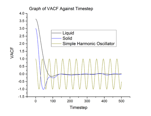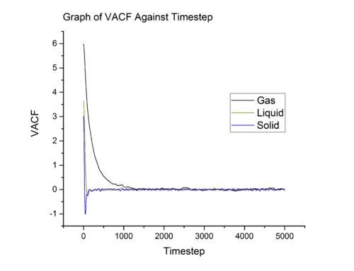
Equation shown above projects velocity at $(t+\tau )$ onto velocity at $\left(t\right)$ and what we obtain is $C\left(\tau \right)$, a number which quantifies the correlation between the two velocities. From gas to solid, the rate of decay of $C\left(\tau \right)$ increases and this is related to the rate of collision. In gas and liquid, particles collide with one another, however, in liquid, the frequency of collision is higher. Rapid exchange of energy between liquid particle causes a liquid particle to lost the initial velocity component at a faster rate than that of gas. From liquid to solid, the situation changes slightly. In a solid, unlike gas and liquid, the particles only vibrate about the equilibrium position. Because the motion of solid particle is confined within a small space, it correlate to initial velocity to a longer period of time. The minima in solid and liquid VACF vs time graph (see Graph 15 and Graph 16) is related to back scattering of particle after collision, hence the $C(\tau )$ is negative in sign (inverse of the initial course).

In simple harmonic oscillator the particles are vibrating about an equilibrium position and there is no collision with another particle, therefore it retain the memory of the initial velocity throughout the simulation. The simple harmonic oscillator aims to illustrate that the velocity correlation in ideal system will continue for infinite amount of time.

Task

Graph 17

Phase Average value of plateau region of graph Diffusion Coefficient from VACF Diffusion Coefficient from MSD Solid (million) 0.000192943 0.000064314 0.000004392 Solid 0.00345 0.00115 0.000892 Liquid (million) 0.25621 0.08540 0.08727 Liquid 0.2316 0.0772 0.0849 Gas (million) 9.8054 3.2685 3.032 Gas 2.44197 0.81399 0.8192

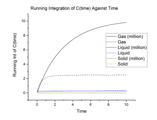The diffusion coefficients calculated using two different methods are in very close agreement and this is expected.

Source of error

According to following equation:

$D=\frac{1}{3}\underset{0}{\overset{\mathrm{\infty }}{\int }}\mathrm{d}\tau ⟨\mathbf{v}\left(0\right)\cdot \mathbf{v}\left(\tau \right)⟩$

The integration range is $0$ to $\mathrm{\infty }$. However in our calculation the integration was stopped at time$=10$, and this could contribute to the error of data. Another source of error is the integration method. By using trapezium rule, we are dividing the graph into different rectangular strips. However, the graph itself can not be be describe perfectly using rectangular strips and will eventually result in overestimation (strips bigger than graph) or underestimation (strips smaller graph).