Rep:Y3CMPCG1417

Section 1 - Introduction to the Ising Model

TASK: Show that the lowest possible energy for the Ising model is $E = - D N J$ , where D is the number of dimensions and N is the total number of spins. What is the multiplicity of this state? Calculate its entropy.

Consider a 1D row of lattice sites of N=3 with spin configuration [+1][+1][+1].

Mathematically the interaction energy is defined asː $- \frac{1}{2} J \sum_{i}^{N} \sum_{j ϵ n e i g h b o u r s (i)}^{} s_{i} s_{j}$ where J is a constant and $s_{i} s_{j}$ is the product between two spins in adjacent lattice sites.

The sum of the interaction energies $\sum_{i}^{N} \sum_{j ϵ n e i g h b o u r s (i)}^{} s_{i} s_{j}$ can be considered as the sum of the individual interaction energies between spinsː $\sum_{i}^{N} \sum_{j ϵ n e i g h b o u r s (i)}^{} s_{i} s_{j} = ϵ_{12} + ϵ_{23} + ϵ_{13} + ϵ_{21} + ϵ_{32} + ϵ_{31}$ .

Although lattice sites 1 and 3 are not adjacent they are said to still interact according to the periodic boundary conditions applied.

However, $ϵ_{12} = ϵ_{21}$ and $ϵ_{23} = ϵ_{32}$ and $ϵ_{13} = ϵ_{31}$ which means that all of the interactions within the system are counted twice, hence the total energy needs to be halved, resulting in the following formula being obtainedː $\sum_{i}^{N} \sum_{j ϵ n e i g h b o u r s (i)}^{} s_{i} s_{j} = 2 ϵ_{12} + 2 ϵ_{13} + 2 ϵ_{23}$ .

It can be determined that $ϵ_{12} = (+ 1) (+ 1) = 1$ , $ϵ_{13} = (+ 1) (+ 1) = 1$ and $ϵ_{23} = (+ 1) (+ 1) = 1$ .

Thereforeː $- \frac{1}{2} J \sum_{i}^{N} \sum_{j ϵ n e i g h b o u r s (i)}^{} s_{i} s_{j} = - \frac{1}{2} J (2 + 2 + 2) = - \frac{1}{2} J 6 = - 3 J = - D N J$ for a 1D lattice with $D = 1$ and 3 lattice sites $N = 3$

The multiplicity of the system, $Ω = \frac{l a t t i c e s i t e s!}{n . s p i n u p! n . s p i n d o w n!}$

Entropy, $S$ is defined as $S = k_{B} l n (Ω)$ and so in this case $S = k_{B} l n (\frac{100!}{100!}) = 0$

TASK: Imagine that the system is in the lowest energy configuration. To move to a different state, one of the spins must spontaneously change direction ("flip"). What is the change in energy if this happens $(D = 3, N = 1000)$ ? How much entropy does the system gain by doing soʔ

In a 3D lattice system, each lattice site has three unique interactions with its neighbours to its left, top and front. In the lowest energy configuration, all spins are parallel and for a system the minimum energy is $E = - D N J$ , so for the system with $N = 1000$ and $D = 3$ , the minimum energy is $- 3000 J$ .

If a single spin is flipped, the product of its spin with its neighbours spin reverses and becomes negative and this increases the total energy of the system. Since 3 unique spin-spin interactions are reversed in sign, the total energy increases by $+ 3 J$ , meaning the new total energy is $- 2997 J$

Initially the multiplicity of the system will be $Ω = \frac{1000!}{1000!}$ , and after the flip, the multiplicity becomes $Ω = \frac{1000!}{999! 1!} = 1000$ .

The associated change in entropy, $Δ S = k_{B} l n (1000) - 0 = 6.91 k_{B}$ , which is an expected increase in entropy as the number of possible configurations of the system increases.

TASK: Calculate the magnetisation of the 1D and 2D lattices in Figure 1. What magnetisation would you expect to observe for an Ising lattice with $D = 3, N = 1000$ at absolute zero?

Figure 1 - Shows 1D (N = 5), 2D (N = 5x5) and 3D (N = 5x5x5) lattices.

Magnetisation is defined as $M = \sum_{i} s_{i}$ . So for the 1D lattice with $N = 5$ in Figure 2, $M = + 1$ and for the 2D lattice with $N = 25, M = + 1$ too.

According to the 3rd Law of thermodynamics, entropy is 0 at absolute zero for a perfect crystalline solid, and consequently it is expected that the lattices will have follow suit and have zero entropy at 0K. To have zero entropy all spins must be parallel as such that magnetisation, $M = N$ . For all the spins to be parallel, there is only one possible configuration. So, for a lattice with $N = 1000$ and $D = 3$ , if $M = N$ , then multiplicity, $Ω = 1$ and entropy, $S = k_{B} l n (1) = 0$ .

Section 2 - Calculating the Energy and Magnetisation

TASK: complete the functions energy() and magnetisation(), which should return the energy of the lattice and the total magnetisation, respectively. In the energy() function you may assume that $J = 1.0$ at all times (in fact, we are working in reduced units in which $J = k_{B}$ , but there will be more information about this in later sections). Do not worry about the efficiency of the code at the moment — we will address the speed in a later part of the experiment.

def magnetisation(self):
		"Return the total magnetisation of the current lattice configuration."
		lat=self.lattice #creates lattice and stores it
		mag=[]
		for i in range(0,len(lat)): #loops through all rows of lattice
			for j in range(0,len(lat[i])): #loops through elements of each row
				mag+=[lat[i][j]] #adds spin value to mag array
		return sum(mag)	#sums all spins from mag array

 def energy(self):
		"Return the total energy of the current lattice configuration."
		
		lat=self.lattice #creates lattice and stores it
		left=[]
		top=[]

		for i in range(0,len(lat)):
			for j in range(0,len(lat[i])):
				left+=[lat[i][j]*lat[i][j-1]] #multiplies spin by spin to left
				top+=[lat[i][j]*lat[i-1][j]] #multiplies spin by spin above it
		int_en=left+top #sums spin products from left and top
		energy=-sum(int_en) #sums all spin products for each spin to give total 

		return energy

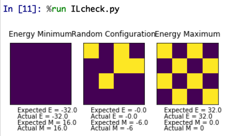
TASK: Run the ILcheck.py script from the IPython Qt console using the command

Figure 2 shows the results when ILcheck.py was ran on my IsingLattice.py file. The ILcheck.py file was ran several times to ensure the code worked for various random lattices.

Section 3 - Introduction to Monte Carlo Simulation

TASK: How many configurations are available to a system with 100 spins? To evaluate these expressions, we have to calculate the energy and magnetisation for each of these configurations, then perform the sum. Let's be very, very, generous, and say that we can analyse $1 \times 1 0^{9}$ configurations per second with our computer. How long will it take to evaluate a single value of ${⟨ M ⟩}_{T}$ ?

For a system with 100 lattice sites and two possible spins for each site, there are $2^{100}$ possible configurations for the system. $2^{100} = 1.27 \times 1 0^{30}$ , so if the computer can analyse $1 \times 1 0^{9}$ configurations per second, then it will take $\frac{1.27 \times 1 0^{30}}{1 0^{9}} = 1.27 \times 1 0^{21} s$ to analyse the whole system, which is longer than the age of the universe and therefore is not a practical approach.

TASK: Implement a single cycle of the above algorithm in the montecarlocycle(T) function. This function should return the energy of your lattice and the magnetisation at the end of the cycle. You may assume that the energy returned by your energy() function is in units of $k_{B}$ ! Complete the statistics() function. This should return the following quantities whenever it is called: $< E >, < E^{2} >, < M >, < M^{2} >$ , and the number of Monte Carlo steps that have elapsed.

E = []
E2 = []
M = []
M2 = []
n_cycles = 0

def montecarlostep(self, T):
		# complete this function so that it performs a single Monte Carlo step
		

		energy = self.energy() #defines initial energy


		#the following two lines will select the coordinates of the random spin for you
		random_i = np.random.choice(range(0, self.n_rows))
		random_j = np.random.choice(range(0, self.n_cols))
		#the following line will choose a random number in the range[0,1) for you
		random_number = np.random.random()

		self.lattice[random_i][random_j]=(self.lattice[random_i][random_j])*(-1) #flips spin and changes lattice
		energy2=self.energy() #energy of new flipped lattice
		deltaE=energy2-energy #calculates change in energy

		#at this point the system has the new spin config and new energy
		
		if deltaE > 0 and random_number > e**(-deltaE/T):
			self.lattice[random_i][random_j]=(self.lattice[random_i][random_j])*(-1) #reverts spin back if rejected else not changed
		
                self.E+=[self.energy()] #records energy
		self.E2+=[self.energy()**2] #records energy squared
		self.M+=[self.magnetisation()] #records magnetisation
		self.M2+=[self.magnetisation()**2] #records magnetisation squared		
		self.n_cycles=self.n_cycles+1 #adds 1 to run total


		return (self.energy(),self.magnetisation())


def statistics(self):
		# complete this function so that it calculates the correct values for the averages of E, E*E (E2), M, M*M (M2), and returns them

		e=np.mean(self.E)
		e2=np.mean(self.E2)
		m=np.mean(self.M)
		m2=np.mean(self.M2)

		return e,e2,m,m2,self.n_cycles

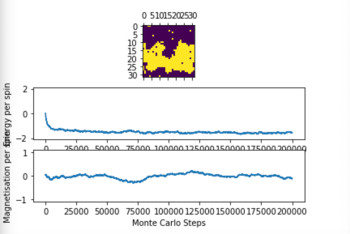
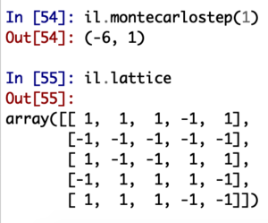
Figure 3 shows the results of a single run of the montecarlostep() function and the lattice the function operated upon.

TASK: If $T < T_{C}$ , do you expect a spontaneous magnetisation (i.e. do you expect $⟨ M ⟩ \neq 0$ )? When the state of the simulation appears to stop changing (when you have reached an equilibrium state), use the controls to export the output to PNG and attach this to your report. You should also include the output from your statistics() function.

If the temperature of the system is less than the Curie Temperature, $T_{C}$ then spontaneous magnetisation can occur and the system will tend to its lowest energy state where all of the spins are parallel - this is a property of ferromagnetic materials.

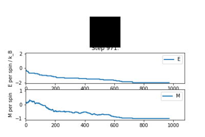
Figure 4 shows that over time the the system spontaneously converges to the minimum energy state with all of the spins parallel to one another and shows, as I expected, that spontaneous magnetisation occurs and also shows that the temperature of this simulation is below the Curie Temperature, $T < T_{C}$ .

Section 4 - Accelerating the Code

TASK: Use the script ILtimetrial.py to record how long your current version of IsingLattice.py takes to perform 2000 Monte Carlo steps. This will vary, depending on what else the computer happens to be doing, so perform repeats and report the error in your average!

Figure 5 show the results of running the ILtimetrial.py file on my code three timesː

Figure 5 - Results of running the ILtimetrial.py file on my code three separate times

This gave me an avergage time of $24.3 s \pm 0.2 s$

TASK: Look at the documentation for the NumPy sum function. You should be able to modify your magnetisation() function so that it uses this to evaluate M. The energy is a little trickier. Familiarise yourself with the NumPy roll and multiply functions, and use these to replace your energy double loop (you will need to call roll and multiply twice!).

 def energy(self):
		"Return the total energy of the current lattice configuration."
		
		left=multiply(roll(self.lattice,1,axis=1),self.lattice) #product of spin with spin left of it
		top=multiply(roll(self.lattice,-1,axis=0),self.lattice) #product of spin with spin above it

		int_en=sum(left+top) #sum of array containing sum of left and top spin products for each spin

		energy = -sum(int_en) #calculates the total energy of system
		return energy

def magnetisation(self):
		"Return the total magnetisation of the current lattice configuration."
		return sum(sum(self.lattice)) #adds up all spins in lattice

The use of the bumpy modules reduces the amount of code required and removes the need for loops making the code significantly shorter, and is therefore expected to run ILtimetrial.py faster than the initial code developed.

TASK: Use the script ILtimetrial.py to record how long your new version of IsingLattice.py takes to perform 2000 Monte Carlo steps. This will vary, depending on what else the computer happens to be doing, so perform repeats and report the error in your average!

Figure 6 shows the result of running the ILtimetrial.py on my new accelerated code.

Figure 6 - Results of running the ILtimetrial.py file on my new updated and accelerated code.

The accelerated code is much faster upon using the roll, multiply and sum modules with a new average time of $0.790 s \pm 0.005$

Section 5 - The effect of temperature

TASK: The script ILfinalframe.py runs for a given number of cycles at a given temperature, then plots a depiction of the final lattice state as well as graphs of the energy and magnetisation as a function of cycle number. This is much quicker than animating every frame! Experiment with different temperature and lattice sizes. How many cycles are typically needed for the system to go from its random starting position to the equilibrium state? Modify your statistics() and montecarlostep() functions so that the first N cycles of the simulation are ignored when calculating the averages. You should state in your report what period you chose to ignore, and include graphs from ILfinalframe.py to illustrate your motivation in choosing this figure.

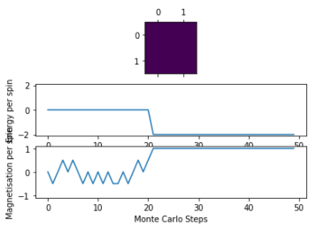
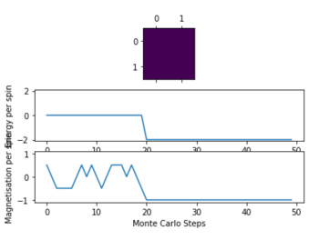
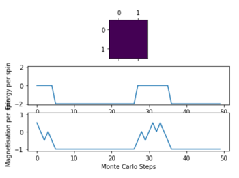
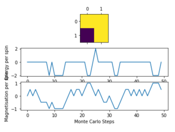
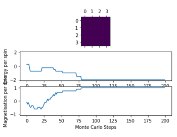
Figure 7 below shows the results from running the ILfinalframe.py for 2x2 lattice at T=1,2,3,5.

Figure 7 - Results of running the ILfinalframe.py file at T=1,2,3,5 for a 2x2 matrix.

For a 2x2 matrix, a suitable cut-off point to exclude from the avergage energies and magnetisations is where the energy and magnetisations per spin are constant, which is 30 steps. For T=3 and T=5 the graphs do not converge because it is possible that these temperatures are higher than the Curie Temperature and as such spontaneous magnetisation will not occur and the system will not diverge to the lowest energy state. At the higher temperatures, there are larger thermal fluctations and the Boltzmann factor is more significant allowing the system to move away from the lowest energy state easier. As a result moving forwards, a suitable cut-off point will only be determined from T=1 and T=2 graphs for the larger matrices.

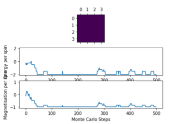
Figure 8 shows the results from running a 4x4 lattice at T=1,2 and 3.

Figure 8 - Results of running the ILfinalframe.py file at T=1,2,3 for a 4x4 matrix.

From Figure 8, a suitable cut-off point for the energy and magnetisations is 200 as this is after where the energy and magnetisation has converged for T=1, and is after the initial large drop in energy for T=2, even though there are a few small fluctuations after 200 steps. The result from T=3 has been included to show the large fluctuations for the larger temperatures, and supporting my choice to determine the cut-off from T=1 and T=2 only.

Figure 9 shows the results for an 8x8 matrix.

Figure 9 - Results of running the ILfinalframe.py file at T=1,2 for an 8x8 matrix

From Figure 9 above, a suitable cut-off point is 1000 steps as this is where the energy and magnetisation has easily converged by and is also the point after which the initial large drop in energy has been overcome for T=2 too.

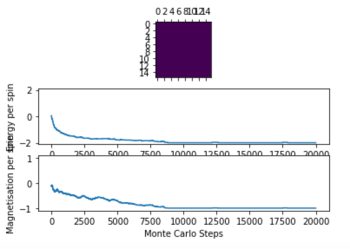
Figure 10 shows the result of running the ILfinalframe.py for a 16x16 matrix.

Figure 10 - Results of running the ILfinalframe.py file at T=1,2 for a 16x16 matrix

From Figure 10, a suitable cut-off point is 15000 steps as for T=1 the energy and magnetisations have converged significantly and will not change much, and likewise this is the same for the T=2 frame.

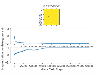
Figure 11 below shows the results from a 32x32 matrix at T=1 and T=2.

Figure 11 - Results of running the ILfinalframe.py file at T=1,2 for a 32x32 matrix

Figure 11 above shows the results of running the ILfinalframe.py file for a 32x32 matrix at T=1 and T=2. As a result a suitable cut-off of 50000 steps was chosen as the energy and magnetisation has significantly converged, but not as much as it could at 100000 steps. I chose a slightly lower value to ensure that the run times of my monte-carlo simulations in future tasks were not extremely time consuming.

The montecarlostep() function was changed by adding a condition that values only above the pre-determined cut-off were included when determining the average value of energy; energy squared; magnetisation and magnetisations squared from the statistics function. The statistics() function did not need to be modified.

The following code is from the 32x32 matrixː

def montecarlostep(self, T):
		# complete this function so that it performs a single Monte Carlo step
		

		energy = self.energy() #defines initial energy


		#the following two lines will select the coordinates of the random spin for you
		random_i = np.random.choice(range(0, self.n_rows))
		random_j = np.random.choice(range(0, self.n_cols))
		#the following line will choose a random number in the range[0,1) for you
		random_number = np.random.random()

		self.lattice[random_i][random_j]=(self.lattice[random_i][random_j])*(-1) #flips spin and changes lattice
		energy2=self.energy() #energy of new flipped lattice
		deltaE=energy2-energy #calculates change in energy

		#at this point the system has the new spin config and new energy
		
		if deltaE > 0 and random_number > e**(-deltaE/T):
			self.lattice[random_i][random_j]=(self.lattice[random_i][random_j])*(-1) #reverts spin back
		

		if self.n_cycles > 50000: #only adds values to array of E,E2,M and M2 above the specific cut-off
			self.E+=[self.energy()]
			self.E2+=[self.energy()**2]
			self.M+=[self.magnetisation()]
			self.M2+=[self.magnetisation()**2]		
		self.n_cycles=self.n_cycles+1

		return (self.energy(),self.magnetisation())

TASK: Use ILtemperaturerange.py to plot the average energy and magnetisation for each temperature, with error bars, for an $8 \times 8$ lattice. Use your intuition and results from the script ILfinalframe.py to estimate how many cycles each simulation should be. The temperature range 0.25 to 5.0 is sufficient. Use as many temperature points as you feel necessary to illustrate the trend, but do not use a temperature spacing larger than 0.5. The NumPy function savetxt() stores your array of output data on disk — you will need it later. Save the file as 8x8.dat so that you know which lattice size it came from.

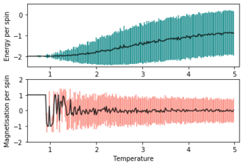
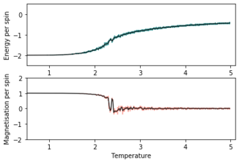
Using the modified code, the file ILtemperaturerange.py was ran on an 8x8 matrix between T=0.5 and T=5 with a step of T=0.02 for 10000 Montecarlo steps and the first 1000 steps of each temperature were excluded when calculating the averages. Figure 12 shows the result of the simulation and also included error bars of standard deviation.

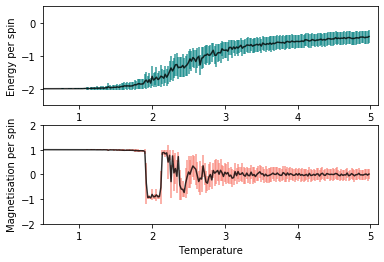
Figure 12 - Graph showing average energy and average magnetisation for an 8x8 lattice with error bars between T=0.5 and T=5

Below is the source code for the script to produce the graph from CG1417IsingModelGraphs.ipynbː

data8x8=np.loadtxt('8x8.dat') #loads data
temps8x8=data8x8[:,0] #stores temperatures
energies8x8=data8x8[:,1] #stores average energy for each T
energysq8x8=data8x8[:,2] #stores average energy squared for each T
mag8x8=data8x8[:,3] #stores magnetisation for each T
magsq8x8=data8x8[:,4] #stores magnetisation squared for each T
stde8x8=data8x8[:,5] #edited ILtemperaturerange.py to record the standard deviation of the energy for each T
stdm8x8=data8x8[:,6] #edited ILtemperaturerange.py to record the standard deviation of the magnetisation for each T

fig = pl.figure()
enerax = fig.add_subplot(2,1,1)
enerax.set_ylabel("Energy per spin")
enerax.set_xlabel("Temperature")
enerax.set_ylim([-2.5, 0.5])
enerax.set_xlim([0.5,5.1])
magax = fig.add_subplot(2,1,2)
magax.set_ylabel("Magnetisation per spin")
magax.set_xlabel("Temperature")
magax.set_ylim([-2, 2])
magax.set_xlim([0.5,5.1])
enerax.errorbar(temps8x8, np.array(energies8x8)/64,yerr=np.divide(stde8x8,64),color='black',ecolor='teal',alpha=0.8) #plots energy per spin against T
magax.errorbar(temps8x8, np.array(mag8x8)/64,yerr=np.divide(stdm8x8,64),alpha=0.8,ecolor='salmon',color='black') #plots magnetisation per spin against T on separate graph
pl.savefig('8x8error.png',bbox_inches='tight') #saves figure
pl.show()

Section 6 - The effect of system size

TASK: Repeat the final task of the previous section for the following lattice sizes: 2x2, 4x4, 8x8, 16x16, 32x32. Make sure that you name each datafile that your produce after the corresponding lattice size! Write a Python script to make a plot showing the energy per spin versus temperature for each of your lattice sizes. Hint: the NumPy loadtxt function is the reverse of the savetxt function, and can be used to read your previously saved files into the script. Repeat this for the magnetisation. As before, use the plot controls to save your a PNG image of your plot and attach this to the report. How big a lattice do you think is big enough to capture the long range fluctuations?

The python script for this section is identical as for the 8x8 graph above in Figure 12 with the relevant files and variables changed accordingly.

Each matrix was simulated using the ILtemperaturerange.py file between T=0.5 and T=5 with a step of T=0.02.

2x2 matrix - 5000 steps, cut-off = 30 steps

4x4 matrix - 1000 steps, cut-off = 200 steps

16x16 matrix - 50000 steps, cut-off = 15000 steps

32x32 matrix - 200000 steps, cut-off = 50000 steps

Figure 13 - Results of running the ILtemperaturerange.py file for 2x2, 4x4, 16x16 and 32x32 matrices.

Long-range interactions are present and more significant in the smaller lattices where there are fewer stronger, short range interactions. As a result, I expect long-range interactions to be important in square lattices up to a 4x4 size.

Section 7 - Determining the Heat Capacity

TASK: By definition, $C = \frac{\partial ⟨ E ⟩}{\partial T}$ . From this, show that $C = \frac{V a r [E]}{k_{B} T^{2}}$ (Where $V a r [E]$ is the variance in $E$ .)

Recall from statistical thermodynamics that the average energy of a system is the sum across all microstates of the probability of that microstate multiplied by the energy of that microstate, which is defined mathematically asː $⟨ E ⟩ = \sum_{i} p_{i} ϵ_{i}$ .

The partition function $q$ is defined as $q = \sum_{i} e x p (- β ϵ_{i})$ where $β = \frac{1}{k_{B} T}$ and the probability, $p_{i}$ can be defined in terms of the partition function as $p_{i} = \frac{e x p (- β ϵ_{i})}{\sum_{i} e x p (- β ϵ_{i})} = \frac{e x p (- β ϵ_{i})}{q}$ .

As a result, $⟨ E ⟩$ can be re-written as $⟨ E ⟩ = \sum_{i} \frac{ϵ_{i} e x p (- β ϵ_{i})}{q} = - \frac{1}{q} \frac{\partial}{\partial β} \sum_{i} e x p (- β ϵ_{i}) = - \frac{1}{q} \frac{\partial q}{\partial β}$

Likewise, $⟨ E^{2} ⟩ = \sum_{i} p_{i} ϵ_{i}^{2} = \sum_{i} \frac{ϵ_{i}^{2} e x p (- β ϵ_{i})}{q} = \frac{1}{q} \frac{\partial^{2}}{\partial β^{2}} \sum_{i} e x p (- β ϵ_{i}) = \frac{1}{q} \frac{\partial^{2} q}{\partial β^{2}}$

From definitionː $V a r [E] = Δ E^{2} = ⟨ E^{2} ⟩ - ⟨ E ⟩^{2}$

When the definition of $⟨ E ⟩$ and $⟨ E^{2} ⟩$ is written in terms of partition function $q$ ː $V a r [E] = ⟨ E^{2} ⟩ - ⟨ E ⟩^{2} = \frac{1}{q} \frac{\partial^{2} q}{\partial β^{2}} - {(\frac{1}{q} \frac{\partial q}{\partial β})}^{2} = \frac{1}{q} \frac{\partial^{2} q}{\partial β^{2}} - \frac{1}{q^{2}} {(\frac{\partial q}{\partial β})}^{2}$ .

According to the chain ruleː $\frac{\partial}{\partial β} (\frac{1}{q} \frac{\partial q}{\partial β}) = \frac{1}{q} \frac{\partial^{2} q}{\partial β^{2}} - \frac{1}{q^{2}} {(\frac{\partial q}{\partial β})}^{2} = - \frac{\partial}{\partial β} ⟨ E ⟩ = V a r [E]$

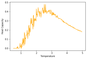
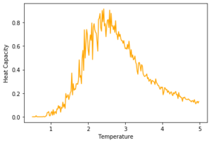
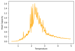
And using the chain rule againː $C = \frac{\partial ⟨ E ⟩}{\partial T} = (- \frac{\partial ⟨ E ⟩}{\partial β}) (- \frac{\partial β}{\partial T}) = \frac{V a r [E]}{k_{B} T^{2}}$

TASK: Write a Python script to make a plot showing the heat capacity versus temperature for each of your lattice sizes from the previous section. You may need to do some research to recall the connection between the variance of a variable, $V a r [X]$ , the mean of its square $⟨ X^{2} ⟩$ , and its squared mean ${⟨ X ⟩}^{2}$ . You may find that the data around the peak is very noisy — this is normal, and is a result of being in the critical region. As before, use the plot controls to save your a PNG image of your plot and attach this to the report.

The python script for this section can be found in the Jupyter Notebook - CG1417IsingModelGraphs.ipynb

2x2 Matrix

4x4 Matrix

8x8 Matrix

16x16 Matrix

32x32 Matrix

Figure 14 - Graphs showing Heat Capacity against Temperature for each matrix size

Here is the source code to produce the figuresː

 def heatCap(energies,energysq,T,latsize):
    #defines the heat capacity for a given temperature
    energiesq=np.multiply(energies,energies) #creates array of (average energies) squared
    varE=np.subtract(energysq,energiesq) #defines variance of average energy
    tempsq=np.multiply(T,T) #array of temperature squared
    return np.array(np.divide(varE,tempsq))/(latsize**2)

heatCap2x2=heatCap(energies2x2,energysq2x2,temps2x2,2) #creates array of heat capacity for each T

fig = pl.figure()
heatcapax = fig.add_subplot(1,1,1)
heatcapax.set_xlabel('Temperature')
heatcapax.set_ylabel('Heat Capacity')
heatcapax.plot(temps2x2,heatCap2x2,color='orange') #plots heat capacity for each T
pl.savefig('cg14172x2heatcap.png',bbox_inches='tight') #saves figure
pl.show()

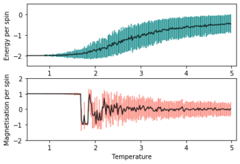
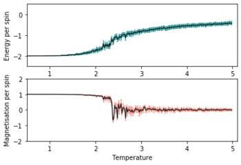
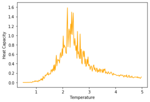
A general trend from the above graphs is that the peak of the graph shifts towards lower temperatures as the size of the matrix used increases which means the Curie Temperature decreases as matrix size increases. Also, as lattice size increases the noise around the peak becomes larger which will affect the accuracy of determining the maximum heat capacity and Curie Temperature for the larger lattices.

Section 8 - Locating the Curie Temperature

TASK: A C++ program has been used to run some much longer simulations than would be possible on the college computers in Python. You can view its source code here if you are interested. Each file contains six columns: $T, E, E^{2}, M, M^{2}, C$ (the final five quantities are per spin), and you can read them with the NumPy loadtxt function as before. For each lattice size, plot the C++ data against your data. For one lattice size, save a PNG of this comparison and add it to your report — add a legend to the graph to label which is which. To do this, you will need to pass the label="..." keyword to the plot function, then call the legend() function of the axis object (documentation here).

The python code used to read and plot the C++ data is found in the Jupyter notebook CG1417IsingModelGraphs.ipynb.

Figure 15 below shows the C++ plotted against my own data for a 16x16 Matrix.

Figure 15 - Graph showing my own data against the C++ data for a 16x16 matrix.

The curves produced using the C++ data are much smoother and have less noise than the data gained from my python code. This is likely due to the C++ code having more montecarlosteps per temperature, reducing the effect of random fluctuations on the averages and also having a smaller step gap which will make the curve smoother as the points are closer together.

Here is the source code the produce the figuresː

#reads data from C++ file
temps2x2C=data2x2C[:,0]
energies2x2C=data2x2C[:,1]
energysq2x2C=data2x2C[:,2]
mag2x2C=data2x2C[:,3]
magsq2x2C=data2x2C[:,4]
heatcap2x2C=data2x2C[:,5]

#fitting C++ data

fig = pl.figure()
enerax = fig.add_subplot(2,1,1)
enerax.set_ylabel("Energy per spin")
enerax.set_xlabel("Temperature")
enerax.set_ylim([-2.5, 0.5])
enerax.set_xlim([0.5,5.1])
magax = fig.add_subplot(2,1,2)
magax.set_ylabel("Magnetisation per spin")
magax.set_xlabel("Temperature")
magax.set_ylim([-2, 2])
magax.set_xlim([0.5,5.1])
enerax.plot(temps2x2, np.array(energies2x2)/4,color='black',alpha=0.7,label='Python Data') #python energy against T
enerax.plot(temps2x2C, energies2x2C, color='red',label='C++ Data') #C energy against T
magax.plot(temps2x2, np.array(mag2x2)/4,color='black',alpha=0.7,label='Python Data') #python magnetisation against T
magax.plot(temps2x2C, mag2x2C,color='red',label='C++ Data') #C energy against T
enerax.legend() #shows legend on energy graph
magax.legend() #shows legend on energy graph
pl.show()

The relevant variables and dat files were changed for each matrix.

TASK: write a script to read the data from a particular file, and plot C vs T, as well as a fitted polynomial. Try changing the degree of the polynomial to improve the fit — in general, it might be difficult to get a good fit! Attach a PNG of an example fit to your report.

The python script to read and plot the fitted polynomial is found in CG1417PolyfitScript.ipynb

Here is the source code for Figure 15

data_test = np.loadtxt("16x16C.dat")
T_test = data_test[:,0] #gets temperatures
C_test = data_test[:,5] #gets heat capacity data

#first we fit the polynomial to the data
fit_test = np.polyfit(T_test, C_test, 35) # fit a polynomial of degree 35ǃ

#now we generate interpolated values of the fitted polynomial over the range of our function
T_min_test = 0.5 #np.min(T_test)
T_max_test = 5 #np.max(T_test)

T_range_test = np.linspace(T_min_test, T_max_test, 1000) #generate 1000 evenly spaced points between T_min and T_max
fitted_C_values_test = np.polyval(fit_test, T_range_test)# use the fit object to generate the corresponding values of C

fig = pl.figure()
heatcapax = fig.add_subplot(1,1,1)
heatcapax.set_xlabel('Temperature')
heatcapax.set_ylabel('Heat Capacity')
heatcapax.plot(T_test,C_test,color='orange',label='C++ Data') #plots C data of heat capacity against temp
heatcapax.plot(T_range_test,fitted_C_values_test,label='Fitted Polynomial') #plots fitted polynomial for whole range of temp
heatcapax.legend()
pl.savefig('FIT_TEST16x16_35.png', bbox_inches='tight') #saves figure
pl.show()

Below in Figure 16 is a plot of my Heat Capacity against Temperature data for a 16x16 matrix and features a polynomial of degree 35 plotted against it. Even with a polynomial of such a high degree, it poorly fits the curve and does not fit to the peak of the curve either.

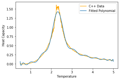
Figure 16 - Plot of Heat Capacity against Temperature along with a poorly fitted polynomial of degree 35.

TASK: Modify your script from the previous section. You should still plot the whole temperature range, but fit the polynomial only to the peak of the heat capacity! You should find it easier to get a good fit when restricted to this region

The script was modified as such that the polynomial was fitted in a set range around the peak of the graph, this is demonstrated in Figure 17 which shows a newly fitted polynomial between a much smaller range of temperatures (T = 2.15-2.55) and a much smaller degree polynomial (3).

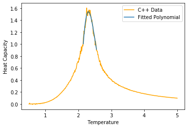
Figure 17 - Graph showing Heat Capacity against Temperature for a 16x16 matrix along with a fitted polynomial between a much more restricted range of temperatures and a significantly lower degree of polynomial

Upon comparison with Figure 16, the new fitted polynomial is a significantly better fit even for a 3rd degree polynomial and is a much more accurate representation of my data around the peak of the graph and will make it easier to determine the maximum value of Heat Capacity. However, the polyfit curve still doesn't perfectly fit the peak due to the significant amount of noise present there.

Here is the source code for Figure 17 from CG1417PolyfitScript.ipynbː

data16 = np.loadtxt("16x16C.dat") #loads data to variable

T16 = data16[:,0] #gets temps
C16 = data16[:,5] # gets heat capacities

Tmin16 = 2.15 #chosen min temp
Tmax16 = 2.55 #chosen max temp

selection16 = np.logical_and(T16 > Tmin16, T16 < Tmax16) #choose only those rows where both conditions are true
peak_T_values16 = T16[selection16] #choose temp values in range chosen above
peak_C_values16 = C16[selection16] #choose heat cap values in range of t above

fit16 = np.polyfit(peak_T_values16,peak_C_values16,3) #fit 3rd order polynomial
peak_T_range16 = np.linspace(Tmin16, Tmax16, 1000) #defines 1000 temps within data range
fitted_C_values16 = np.polyval(fit16, peak_T_range16) #use the fit object to get corresponding values of heat cap

fig = pl.figure()
heatcapax = fig.add_subplot(1,1,1)
heatcapax.set_xlabel('Temperature')
heatcapax.set_ylabel('Heat Capacity')
heatcapax.plot(T16,C16,color='orange',label='C++ Data') #plots C data of heat cap against temp
heatcapax.plot(peak_T_range16,fitted_C_values16,label='Fitted Polynomial') #plots fitted polynomial for small range
heatcapax.legend()
pl.savefig('FIT_16x16C_3.png', bbox_inches='tight') #saves figure
pl.show()

TASK: find the temperature at which the maximum in C occurs for each datafile that you were given. Make a text file containing two colums: the lattice side length (2,4,8, etc.), and the temperature at which C is a maximum. This is your estimate of $T_{C}$ for that side length. Make a plot that uses the scaling relation given above to determine $T_{C, \infty}$ . By doing a little research online, you should be able to find the theoretical exact Curie temperature for the infinite 2D Ising lattice. How does your value compare to this? Are you surprised by how good/bad the agreement is? Attach a PNG of this final graph to your report, and discuss briefly what you think the major sources of error are in your estimate.

Figure 18 below shows a graph of $T_{C, L}$ against $\frac{1}{L a t t i c e S i z e}$ to determine the Curie Temperature of an infinite 2D Ising Model Lattice $T_{C, \infty}$ . The black dots represent the raw data obtained from obtaining the temperature at which the Heat Capacity was a maximum for the lattices and the red line in a linear curve fit plotted against the data to allow the y-intercept which is the Curie Temperature for the infinite 2D lattice to be determined.

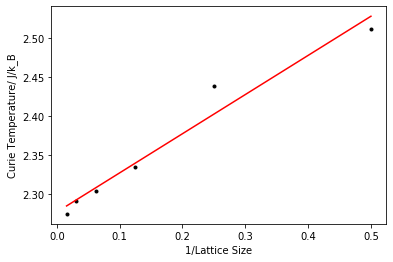
Figure 18 - Plot of 1/Lattice Size against Curie Temperature for that lattice size.

The value for $T_{C, \inf}$ obtained from the data is $T_{C, \infty} = 2.277 \frac{J}{k_{B}}$ with a literature value being $T_{C, \infty} = 2.269 \frac{J}{k_{B}}$ ^[1]for an infinite square 2D lattice. This means that my result slightly over-estimates the Curie Temperature for the infinite lattice and as a result for an infinite lattice the temperature at which spontaneous magnetisation stops would actually occur at a slightly lower temperature than expected. However, the difference between my value and the literature value is only 0.008 which is incredibly small and the amount of agreement between the two values is somewhat surprising, which means that the error in my estimates of the Curie Temperature for each lattice size is relatively small. The points which have the largest residuals and deviation from the line of best fit in Figure 17 corresponds to the smaller lattice sizes of 2x2 and 4x4 where longer range interactions are more significant. The longer range interactions posed by the boundary conditions are significant for the smaller sizes and causes the energy of the smaller matrices to be less accurate and have a larger associated error with the energy and the Curie Temperature for that lattice size. This affects the accuracy of the line of best fit and to increase the accuracy of this line, larger lattice sizes of 128x128, 256x256 etc should be included in the calculation for the line of best fit and the smaller matrices ignored - this should allow a more accurate value of $T_{C, \infty}$ to be determined.

Below is the source code used to generate Figure 18 from CG1417PolyfitScript.py

Cmax64x64 = np.max(fitted_C_values64) #finds Cmax for 64x64 matrix - done for others already 
Tmax64x64 = peak_T_range64[fitted_C_values64 == Cmax64x64] #finds Tmax corresponding to Cmax

LatSize=[2,4,8,16,32,64] #stores lattice sizes
Tmax=[Tmax2x2,Tmax4x4,Tmax8x8,Tmax16x16,Tmax32x32,Tmax64x64] #stores corresponding Tmax data
np.savetxt('CmaxVSTmax.txt', (LatSize,Tmax)) #writes data to txt file

ScalData=np.loadtxt('CmaxVSTmax.txt') #loads data
LatticeSize=ScalData[0] #gets lattice sizes
TempMax=ScalData[1] #gets max temp or curie temp for each lattice

Lmin1min = np.min(np.divide(1,LatticeSize)) #minimum of 1/LatticeSize values
Lmin1max = np.max(np.divide(1,LatticeSize)) #maximum of 1/LatticeSize values

fitTcl = np.polyfit(np.divide(1,LatticeSize),TempMax, 1) #creates fit object

Lmin1values = np.linspace(Lmin1min, Lmin1max, 1000) #finds 1000 values between min and max x-axis value of 1/LatticeSize
fitted_Tcl_values = np.polyval(fitTcl, Lmin1values) #creates corresponding Curie Temp values for each value in Lmin1values

fig = pl.figure()
scalrelax = fig.add_subplot(1,1,1)
scalrelax.set_xlabel('1/Lattice Size')
scalrelax.set_ylabel('Curie Temperature/ J/k_B')
scalrelax.plot(np.divide(1,LatticeSize),TempMax,color='black',marker='.',linestyle='') #plots Curie Temp against 1/LatticeSize
scalrelax.plot(Lmin1values,fitted_Tcl_values,color='red',marker='',linestyle='-') #plots line of best fit for data above
pl.savefig('CurieTemp.png', bbox_inches='tight') #saves figure
pl.show()

References

↑ L. Onsager, Phys. Rev., 1944, 65, 117--149.

[1] L. Onsager, Phys. Rev., 1944, 65, 117--149.

[1]