Rep:Wm1415CMPbackup

This is William Micou's report on the compulsory CMP experiment: Ising Model.

Introduction to the Ising Model

TASK: Show that the lowest possible energy for the Ising model is $E = - D N J$ , where $D$ is the number of dimensions and $N$ is the total number of spins. What is the multiplicity of this state? Calculate its entropy.

In the absence of an external magnetic field, the energy of the lattice depends on the interaction energy $E$ between adjacent sites^[1]:

E = - \frac{1}{2} J \sum_{i}^{N} \sum_{j \in n e i g h b o u r s (i)} s_{i} s_{j}

Thus, the energy is minimised when neighbouring spins are aligned. $J$ is the exchange energy and comes about from the Pauli Exclusion Principle^[2]: electrons cannot occupy the same quantum state. Electrons on neighbouring atoms with spins aligned cannot occupy the same space - electron repulsion is reduced and the total energy is lowered^[2].

The state with the lowest possible energy is the state with all spins aligned. To calculate its energy, the total number of interactions must be counted.

For an infinite lattice, there are 2 nearest neighbours per dimension (degree of freedom): number of pairs of interactions $= 2 N D$ .

Hence, total number of interactions $= \frac{1}{2} \times 2 N D = N D$ .

Since all spins are aligned, every interaction will contribute $- J$ to the energy:

$E = - J \times N D = - D N J$ as required.

This lowest energy state is comprised of 2 microstates: all spins up, and all spins down. Thus, the entropy $S$ is:

$S = k_{B} \ln Ω = k_{B} \ln 2$

TASK: Imagine that the system is in the lowest energy configuration. To move to a different state, one of the spins must spontaneously change direction ("flip"). What is the change in energy if this happens ( $D = 3, N = 1000$ )? How much entropy does the system gain by doing so?

Lowest energy state is -3000J

The spin being flipped has 6 nearest neighbours. Its 6 interactions with the lattice contribute -6J to the energy. After flipping, the spin now contributes +6J to the energy.

Energy of one spin flipped state: -2988J

Difference of +12J

There are 2000 microstates for this system: 1000 all but one spin up states, or 1000 all but one spin down states.

$S = k_{B} \ln Ω = k_{B} \ln 2000 - k_{B} \ln 2 = k_{B} \ln 1000$

TASK: Calculate the magnetisation of the 1D and 2D lattices in figure 1. What magnetisation would you expect to observe for an Ising lattice with $D = 3, N = 1000$ at absolute zero?

1D lattice: magnetisation = +1

2D lattice: magnetisation = +1

At absolute zero, entropic effects vanish and the system will remain in the lowest energy state, with all spins aligned. Thus the magnetisation would be either +N or -N (+1000 or -1000).

Calculating the energy and magnetisation

TASK: complete the functions energy() and magnetisation(), which should return the energy of the lattice and the total magnetisation, respectively. In the energy() function you may assume that $J = 1.0$ at all times (in fact, we are working in reduced units in which $J = k_{B}$ , but there will be more information about this in later sections). Do not worry about the efficiency of the code at the moment — we will address the speed in a later part of the experiment.

Below is the initial, inefficient code for energy() and magnetisation() using indented for loops.

    def energy(self):
        "Return the total energy of the current lattice configuration."
        energy = 0.0
        for i in range(0,self.n_rows):
            for j in range(0,self.n_cols):
        		start = int(self.lattice[i][j])
        		top = int(self.lattice[i-1][j])
        		bot = int(self.lattice[(i+1)%self.n_rows][j])
        		left = int(self.lattice[i][j-1])
        		right = int(self.lattice[i][(j+1)%self.n_cols])
        		total_interaction = (start*top)+(start*bot)+(start*left)+(start*right)
         		energy = energy + (-0.5*total_interaction)
        return energy

    def magnetisation(self):
        "Return the total magnetisation of the current lattice configuration."
        magnetisation = 0
        for i in range(0,self.n_rows):
        	for j in range(0,self.n_cols):
        		magnetisation = magnetisation + int(self.lattice[i][j])
        return magnetisation

The energy() method loops over every spin in the lattice and adds up every interaction. The modulus allows for boundary conditions for spins at the edges of our lattice. The magnetisation() method simply adds up every spin value in the lattice.

TASK: Run the ILcheck.py script from the IPython Qt console using the command

%run ILcheck.py

The displayed window has a series of control buttons in the bottom left, one of which will allow you to export the figure as a PNG image. Save an image of the ILcheck.py output, and include it in your report.

Introduction to the Monte Carlo simulation

TASK: How many configurations are available to a system with 100 spins? To evaluate these expressions, we have to calculate the energy and magnetisation for each of these configurations, then perform the sum. Let's be very, very, generous, and say that we can analyse $1 \times 1 0^{9}$ configurations per second with our computer. How long will it take to evaluate a single value of ${⟨ M ⟩}_{T}$ ?

For a system of 100 spins, there are $2^{100}$ configurations. Evaluating $1 0^{9}$ calculations per second, it would take around $1.3 \times 1 0^{21}$ seconds to finish the calculation - around 4 orders of magnitude larger than the age of the Universe. Clearly, this is impractical: importance sampling is a method of circumventing this.

TASK: Implement a single cycle of the above algorithm in the montecarlocycle(T) function. This function should return the energy of your lattice and the magnetisation at the end of the cycle. You may assume that the energy returned by your energy() function is in units of $k_{B}$ ! Complete the statistics() function. This should return the following quantities whenever it is called: $< E >, < E^{2} >, < M >, < M^{2} >$ , and the number of Monte Carlo steps that have elapsed.

    def montecarlostep(self, T):
        "Performs a single cycle of the Monte Carlo algorithm presented in the lab script."
        # first: increase the number of steps elapsed
        self.n_cycles = self.n_cycles + 1
        # introduce a variable that will indicate whether the new configuration should be rejected or kept
        accept_configuration = True
        # energy of the original lattice (E_0)
        energy_0 = self.energy()
        # select coordinates for a random spin in the lattice
        random_i = np.random.choice(range(0, self.n_rows))
        random_j = np.random.choice(range(0, self.n_cols))
        # flip the spin in the lattice
        self.lattice[random_i, random_j] = -1 * self.lattice[random_i, random_j]
        # calculate new lattice energy (E_1)
        energy_1 = self.energy()
        # calculate the difference in energy
        delta = energy_1 - energy_0
        # if the new configuration is lower in energy, keep the new configuration
        if delta < 0:
            accept_configuration = True

        # choose a random number in the range [0,1)
        random_number = np.random.random()
        boltzmann_factor = np.exp(-delta / T)
        # if the new configuration is higher in energy, compare random number to Boltzmann factor
        if delta >= 0:
            if random_number <= boltzmann_factor:
                accept_configuration = True
            else:
                accept_configuration = False

        if accept_configuration == False:
            # return to original lattice
            self.lattice[random_i, random_j] = -1 * self.lattice[random_i, random_j]

        # keep running totals of data for n_cycles > 250000 steps
        discount = 250000
        if self.n_cycles > discount:
            self.E = self.E + self.energy()
            self.E2 = self.E2 + (self.energy()) ** 2
            self.M = self.M + self.magnetisation()
            self.M2 = self.M2 + (self.magnetisation()) ** 2
        # return the post-MMC step energy and magnetisation as a list
        return [self.energy(), self.magnetisation()]

    def statistics(self):
        "Calculates the average values of E, E*E (E2), M, M*M(M2) and returns them."
        # Discount the first 250000 steps.
        discount = 250000
        avg_E = self.E / (self.n_cycles-discount)
        avg_E2 = self.E2 / (self.n_cycles-discount)
        avg_M = self.M / (self.n_cycles-discount)
        avg_M2 = self.M2 / (self.n_cycles-discount)
        return [avg_E, avg_E2, avg_M, avg_M2, self.n_cycles]

This code comes from later in the assignment - when the methods are modified to discard the first 250000 steps from the running averages of energy and magnetisation.

TASK: If $T < T_{C}$ , do you expect a spontaneous magnetisation (i.e. do you expect $⟨ M ⟩ \neq 0$ )? When the state of the simulation appears to stop changing (when you have reached an equilibrium state), use the controls to export the output to PNG and attach this to your report. You should also include the output from your statistics() function.

The original ILanim.py expected only 4 entries from the statistics() method:

    E, E2, M, M2 = il.statistics()
    print("Averaged quantities:")
    print("E = ", E/spins)
    print("E*E = ", E2/spins/spins)
    print("M = ", M/spins)
    print("M*M = ", M2/spins/spins)

I modified the code to expect 5 entries from the statistics() method, which also outputs the number of cycles elapsed:

    E, E2, M, M2, n = il.statistics()
    print("Averaged quantities:")
    print("E = ", E/spins)
    print("E*E = ", E2/spins/spins)
    print("M = ", M/spins)
    print("M*M = ", M2/spins/spins)
    print("No. cycles = ", n)

The figure below shows the outcome of running ILanim.py for an 8x8 lattice, at temperature = 1. This is below the critical temperature: the figure shows the system converged to the lowest energy state, with all spins aligned. The atoms do not have sufficient thermal energy to flip their spins: the exchange effect dominates over the entropic effect at low temperatures - spontaneous magnetisation is expected.

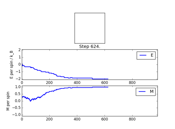
The output of statistics():

    Averaged quantities:
    E =  -1.44239045383
    E*E =  2.44085607394
    M =  0.732834507042
    M*M =  0.641262287265
    No. cycles =  639

These are averaged quantities over the course of the rearrangement of the lattice: no cycles were discarded in the calculation of the averages (discount variable set to zero).

Accelerating the code

TASK: Use the script ILtimetrial.py to record how long your current version of IsingLattice.py takes to perform 2000 Monte Carlo steps. This will vary, depending on what else the computer happens to be doing, so perform repeats and report the error in your average!

9.74 $\pm$ 0.26 seconds before optimisation (10 trials)

TASK: Look at the documentation for the NumPy sum function. You should be able to modify your magnetisation() function so that it uses this to evaluate M. The energy is a little trickier. Familiarise yourself with the NumPy roll and multiply functions, and use these to replace your energy double loop (you will need to call roll and multiply twice!).

    def energy(self):
        "Return the total energy of the current lattice configuration."
        # Roll the lattice vertically and multiply with original to find total vertical interactions
        vertical_interactions = np.multiply(self.lattice, np.roll(self.lattice, 1, axis=0))
        # Roll the lattice horizontally and multiply with original to find total horizontal interactions
        horizontal_interactions = np.multiply(self.lattice, np.roll(self.lattice, 1, axis=1))
        return (-1)*(np.sum(vertical_interactions + horizontal_interactions))

    def magnetisation(self):
        "Return the total magnetisation of the current lattice configuration."
        # Sum every spin in the lattice to obtain the total magnetisation.
        return np.sum(self.lattice)

TASK: Use the script ILtimetrial.py to record how long your new version of IsingLattice.py takes to perform 2000 Monte Carlo steps. This will vary, depending on what else the computer happens to be doing, so perform repeats and report the error in your average!

0.21 $\pm$ 0.01 seconds after second optimisation (10 trials) (new code)

The effect of temperature

TASK: The script ILfinalframe.py runs for a given number of cycles at a given temperature, then plots a depiction of the final lattice state as well as graphs of the energy and magnetisation as a function of cycle number. This is much quicker than animating every frame! Experiment with different temperature and lattice sizes. How many cycles are typically needed for the system to go from its random starting position to the equilibrium state? Modify your statistics() and montecarlostep() functions so that the first N cycles of the simulation are ignored when calculating the averages. You should state in your report what period you chose to ignore, and include graphs from ILfinalframe.py to illustrate your motivation in choosing this figure.

Lattice	Temperature	ILfinalframe.py	Comments
6x6	1.0		System stabilises after ~170 steps
8x8	1.0		System stabilises after 600-700 steps
8x8	2.0		System stabilises after ~2600 steps
8x8	3.0		Above the critical temperature: spins flip rapidly and the system starts fluctuating from the first step.
10x10	0.5		System stabilises after ~1800 steps
10x10	1.5		System stabilises after ~2200 steps
10x10	3.0		Above the critical temperature: spins flip rapidly and the system starts fluctuating from the first step.
15x15	1.0		Magnetisation appears to converge after 1-2000 steps, but then much later on the final state is found.
32x32	0.5	'Clumping' No 'clumping'	The larger 32x32 lattice can either find the lowest possible energy state, or get stuck in a metastable clumped state - even with the same initial conditions.
32x32	1.0	'Clumping' No 'clumping'	The larger 32x32 lattice can either find the lowest possible energy state, or get stuck in a metastable clumped state - even with the same initial conditions.
32x32	3.0		Above the critical temperature, the larger 32x32 lattice reaches a 'final' state after around 5000 steps: many more steps required cf smaller lattices.

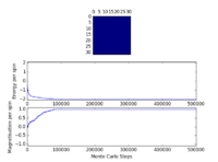
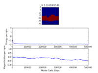
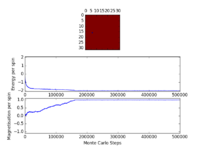
The number of steps required to converge to the 'final' state increases with lattice size. Consider the case below the critical temperature - we expect to observe spontaneous magnetisation and for all spins to align. For larger lattices, it may take many steps to flip the remaining sites since they are chosen entirely at random - and the probability of choosing the 'correct' site to flip decreases with lattice size. For the smaller lattice sizes (<16x16), the system behaves as expected within at most a few thousand steps.

Larger lattices are prone to 'clumping' - the entire system is not in the same spin state, but large regions of spin-aligned atoms form. These are metastable states: spins have aligned within the clump to lower the energy, but there is not enough thermal energy in the system to break up neighbouring clumps of opposing spins. A local minimum of the PES has been found, but the global minimum requires crossing an activation barrier. A good example of this is the 32x32 lattice above: using exactly the same conditions, the system can either reach the lowest possible energy state or show clumping.

For the effect of temperature, consider the 8x8 lattice shown above. Well below the critical temperature, there is not sufficient thermal energy to cause large fluctuations in the spin states of the system and spontaneous magnetisation occurs quickly. Approaching the critical temperature, more fluctuations are possible, and more steps are required for the system to finally reach the lowest possible energy state. Above the critical temperature, spontaneous magnetisation no longer occurs, and entropic effects start to dominate - from the first step the entire system is fluctuating rapidly.

TASK: Use ILtemperaturerange.py to plot the average energy and magnetisation for each temperature, with error bars, for an $8 \times 8$ lattice. Use your initution and results from the script ILfinalframe.py to estimate how many cycles each simulation should be. The temperature range 0.25 to 5.0 is sufficient. Use as many temperature points as you feel necessary to illustrate the trend, but do not use a temperature spacing larger than 0.5. T NumPy function savetxt() stores your array of output data on disk — you will need it later. Save the file as 8x8.dat so that you know which lattice size it came from.

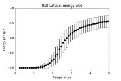
The experiment runs for 500000 steps, with the first 250000 steps discarded from the calculation of the average energies. This is a compromise between allowing the larger lattice systems a better chance of converging to the final state, and running the experiment on a reasonable timescale. The results from the 8x8 lattice, with error bars:

The effect of system size

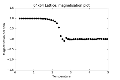
TASK: Repeat the final task of the previous section for the following lattice sizes: 2x2, 4x4, 8x8, 16x16, 32x32. Make sure that you name each datafile that your produce after the corresponding lattice size! Write a Python script to make a plot showing the energy per spin versus temperature for each of your lattice sizes. Hint: the NumPy loadtxt function is the reverse of the savetxt function, and can be used to read your previously saved files into the script. Repeat this for the magnetisation. As before, use the plot controls to save your a PNG image of your plot and attach this to the report. How big a lattice do you think is big enough to capture the long range fluctuations?

Lattice Size	Energy plot	Magnetisation plot
2x2
4x4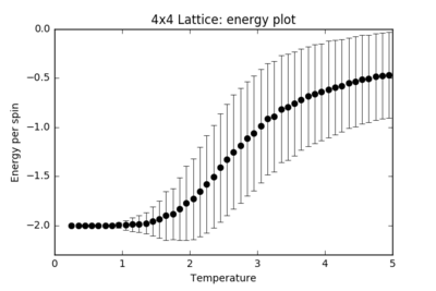
8x8
16x16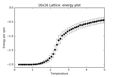
32x32
64x64
All

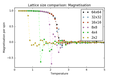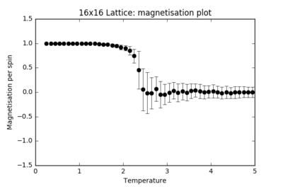
For each finite lattice size plot, there is a noticeable trend in the size of the error bars. These represent the number of energy and magnetisation states available at each temperature. Far below $T_{C}$ , the error bars are almost negligible: there is spontaneous magnetisation and there is not sufficient thermal energy in the system to overcome the activation barrier in flipping the spins. From around T = 1.5, more states become accessible to the system and the error bars steadily increase in size until the critical temperature is reached, where the system undergoes a secondary phase transition and the error bars are at their largest: the states available at this temperature span the largest range of energies and magnetisations. At $T > T_{C}$ , the system has enough thermal energy to undergo fluctuations and the error bars remain considerably large.

As the size of the lattice increases, the size of the error bars decrease. For a 2x2 lattice, a single spin flip represents a huge change in the energy and magnetisation of the whole system. For a 64x64 lattice, the difference in energy and magnetisation for the whole system when a single spin flips is almost negligible. The fluctuations result in smaller fractional changes in the system as the lattice size increases, hence the error bars decrease.

When plotted on the same graph, the energy and magnetisation plots appear to converge for the higher lattice sizes. The 16x16 and higher lattices are big enough to capture the long-range fluctuations: a single spin flip brings about a finer change in the whole system's energy.

Determining the heat capacity

TASK: By definition,

$C = \frac{\partial ⟨ E ⟩}{\partial T}$

From this, show that

$C = \frac{V a r [E]}{k_{B} T^{2}}$

(Where $V a r [E]$ is the variance in $E$ .)

The average energy can be related to the partition function^[3], $Z = \sum \exp (- β ε_{i})$ , with $β = \frac{1}{k_{B} T}$ and $ε_{i}$ being the energy of each state $i$ :

⟨ E ⟩ = \frac{E}{N} = \frac{1}{N} \sum N_{i} ε_{i} = \frac{1}{Z} \sum ε_{i} \exp (- β ε_{i}) = - \frac{1}{Z} \frac{\partial Z}{\partial β} = - \frac{\partial \ln Z}{\partial β}

Similarly, the expectation value for $⟨ E^{2} ⟩$ can be calculated from the partition function:

⟨ E^{2} ⟩ = \sum ε_{i}^{2} p_{i} = \frac{\sum ε_{i}^{2} \exp (- β ε_{i})}{\sum \exp (- β ε_{i})} = \frac{1}{Z} \frac{\partial^{2}}{\partial β^{2}} [\sum \exp (- β ε_{i})] = \frac{1}{Z} \frac{\partial^{2} Z}{\partial β^{2}}

Variance, $V a r [E]$ , can be expressed as:

V a r [E] = ⟨ E^{2} ⟩ - ⟨ E ⟩^{2}

V a r [E] = \frac{1}{Z} \frac{\partial^{2} Z}{\partial β^{2}} - {(- \frac{1}{Z} \frac{\partial Z}{\partial β})}^{2}

Let us show that this expression for variance is equivalent to $\frac{\partial}{\partial β} (\frac{1}{Z} \frac{\partial Z}{\partial β})$ :

\frac{\partial}{\partial β} (\frac{1}{Z} \frac{\partial Z}{\partial β}) = \frac{1}{Z} \frac{\partial^{2} Z}{\partial β^{2}} + \frac{\partial (\frac{1}{Z})}{\partial β} \frac{\partial Z}{\partial β} = \frac{1}{Z} \frac{\partial^{2} Z}{\partial β^{2}} + (\frac{\partial (\frac{1}{Z})}{\partial Z} \frac{\partial Z}{\partial β}) \frac{\partial Z}{\partial β} = \frac{1}{Z} \frac{\partial^{2} Z}{\partial β^{2}} - \frac{1}{Z^{2}} {(\frac{\partial Z}{\partial β})}^{2} = V a r [E]

Hence:

V a r [E] = \frac{\partial}{\partial β} (\frac{1}{Z} \frac{\partial Z}{\partial β}) = \frac{\partial^{2} \ln Z}{\partial β^{2}}

But, since $⟨ E ⟩ = - \frac{\partial \ln Z}{\partial β}$ , and $\frac{\partial}{\partial β} = \frac{\partial T}{\partial β} \frac{\partial}{\partial T} = (\frac{1}{\frac{\partial β}{\partial T}}) \frac{\partial}{\partial T} = (- k_{B} T^{2}) \frac{\partial}{\partial T}$ , the above can be rewritten as^[3]:

V a r [E] = \frac{\partial^{2} \ln Z}{\partial β^{2}} = - \frac{\partial}{\partial β} (- \frac{\partial \ln Z}{\partial β}) = - \frac{\partial}{\partial β} ⟨ E ⟩ = - (- k_{B} T^{2} \frac{\partial}{\partial T}) ⟨ E ⟩ = k_{B} T^{2} C_{V}

Therefore:

C_{V} = \frac{V a r [E]}{k_{B} T^{2}}

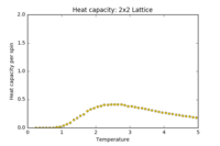
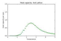
TASK: Write a Python script to make a plot showing the heat capacity versus temperature for each of your lattice sizes from the previous section. You may need to do some research to recall the connection between the variance of a variable, $V a r [X]$ , the mean of its square $⟨ X^{2} ⟩$ , and its squared mean ${⟨ X ⟩}^{2}$ . You may find that the data around the peak is very noisy — this is normal, and is a result of being in the critical region. As before, use the plot controls to save your a PNG image of your plot and attach this to the report.

2x2 Heat Capacity	4x4 Heat Capacity	8x8 Heat Capacity	16x16 Heat Capacity	32x32 Heat Capacity	64x64 Heat Capacity	Combined

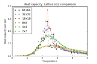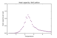
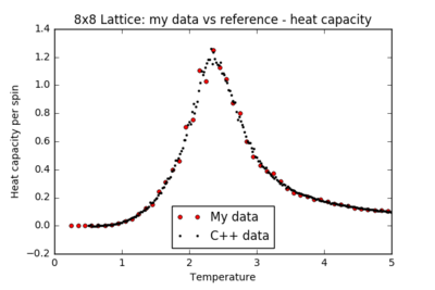
These plots show the heat capacities for each lattice size, using the same data from the previous section. In all cases, the regions $T < < T_{C}$ and $T > > T_{C}$ are well-resolved, and in the next section it will be shown that they map to the reference C++ data perfectly. However, in the region of the critical temperature, larger lattices give a very noisy plot. Further repeats of larger lattices at the critical temperature will be explored later in the report.

The last plot, showing the heat capacity curves for all lattice sizes, somewhat demonstrates an equation stated in the lab script, relating the temperature at which heat capacity is maximised with lattice size:

T_{C, L} = \frac{A}{L} + T_{C, \infty}

From this, one would expect the peak in the heat capacity to shift to lower temperatures as the lattice size increases. This can be seen up to the 8x8 lattice: above this, only one repeat of the experiment is not sufficient to accurately map the critical region and the trend is not clear for this example.

Locating the Curie temperature

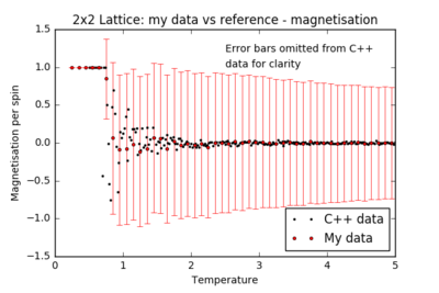
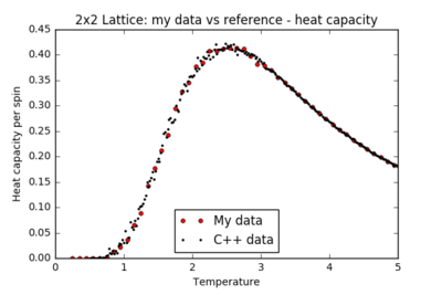
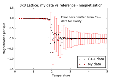
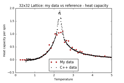
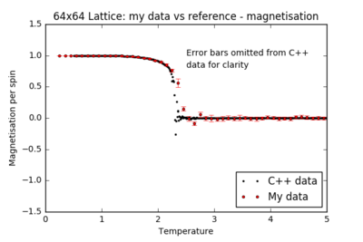
TASK: A C++ program has been used to run some much longer simulations than would be possible on the college computers in Python. You can view its source code here if you are interested. Each file contains six columns: $T, E, E^{2}, M, M^{2}, C$ (the final five quantities are per spin), and you can read them with the NumPy loadtxt function as before. For each lattice size, plot the C++ data against your data. For one lattice size, save a PNG of this comparison and add it to your report — add a legend to the graph to label which is which. To do this, you will need to pass the label="..." keyword to the plot function, then call the legend() function of the axis object (documentation here).

Lattice Size	Energy: Python vs C++	Magnetisation: Python vs C++	Heat Capacity: Python vs C++
2x2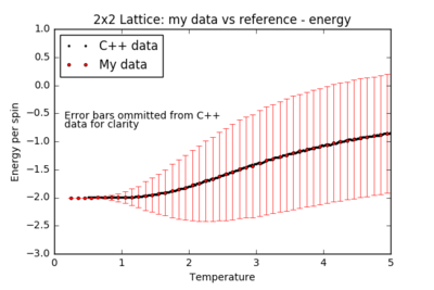
4x4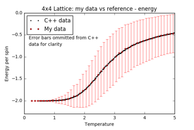
8x8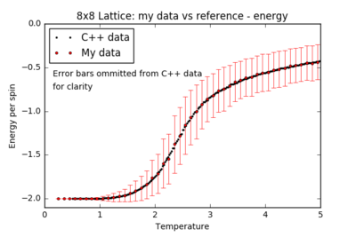
16x16
32x32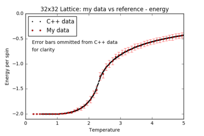
64x64

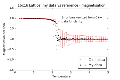
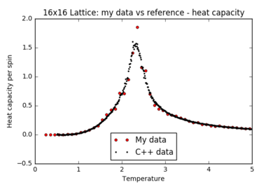
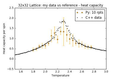
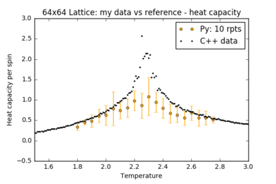
For all lattice sizes, the energy and magnetisation are in agreement with the reference C++ data. The heat capacity plots also match the reference for smaller lattice sizes, producing a smooth curve with almost no noise: the system is small enough to probe all the possible configurations. However, there is substantial noise in the heat capacity for larger lattices (16x16 and above) in the region of the critical temperature: one repeat of the experiment is not sufficient to accurately model the many possible mechanisms of phase transition.

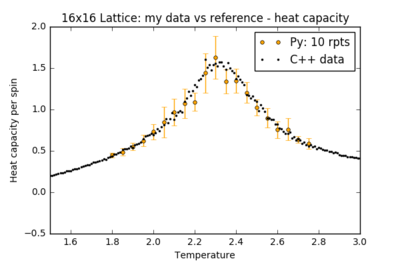
The relaxation process for a random lattice configuration can be described by a free energy surface. The path whereby the system relaxes depends on the initial configuration - which, in our model, is random. Thus, for each run of the experiment, a different section of the free energy surface is explored: the local minimum where the system stabilises will have a different energy in the different paths taken. The activation barriers between local minima are mediated by 'clumping': regions of spin-aligned lattice sites form, which are unfavourable to disrupt. In the critical temperature region, there is not sufficient thermal energy to eliminate clumping: as a result, there are many metastable states the system can relax to, each with different energies. This results in a large number of possible configurations, and hence a noisy plot of energy, magnetisation and heat capacity.

To reduce the noise, more repeats must be performed and the results averaged to sample more relaxation paths on the free energy surface. The figures below show the results of further simulations run in the critical temperature range for larger lattices, with a comparison between a single run of the experiment and an averaged plot from 10 repeats. Error bars in the heat capacity plot were obtained by calculating the standard deviation across repeats.

Lattice Size	Heat Capacity: Single run	Heat Capacity: 10 repeats
16x16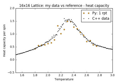
32x32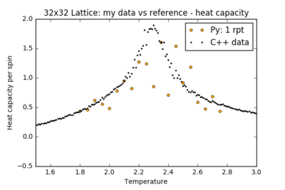
64x64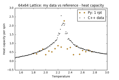

Even with these repeat experiments, the values for the heat capacity for the larger 32x32 and 64x64 lattices seem to be consistently smaller than the reference data at the critical temperature. Perhaps this is because the system is not being given enough steps to fully explore the potential energy surface. All these plots have been using the same method for this report - discounting the first 250,000 steps and recording the next 250,000. To test this, an additional run of the 32x32 lattice was performed: discounting the first 250,000 steps and recording the next 1,250,000 steps:

As this was computationally very expensive, only one repeat was manageable for the timescale of this experiment. While it may not be scientifically rigorous to draw any conclusions from one repeat of an experiment which depends on chance, this figure is certainly promising - the extra steps seem to have alleviated the underestimation of the heat capacity - and a closer match to the C++ data may be obtained with further repeats. Unfortunately, this was not investigated further due to time constraints of the experiment.

To extract the Curie temperature, the reference data - with clearly resolved peaks in the heat capacity - will be examined first, and then compared to the value obtained from the data generated in Python.

Locating the Curie temperature - Reference C++ data

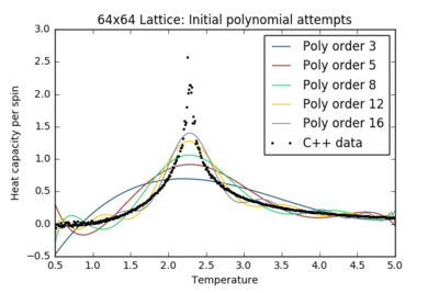
TASK: write a script to read the data from a particular file, and plot C vs T, as well as a fitted polynomial. Try changing the degree of the polynomial to improve the fit — in general, it might be difficult to get a good fit! Attach a PNG of an example fit to your report.

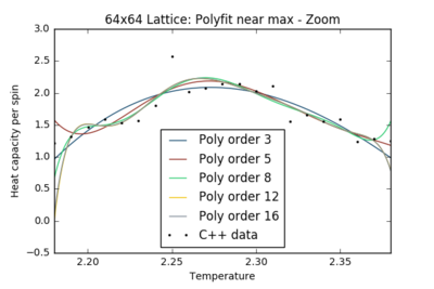
TASK: Modify your script from the previous section. You should still plot the whole temperature range, but fit the polynomial only to the peak of the heat capacity! You should find it easier to get a good fit when restricted to this region.

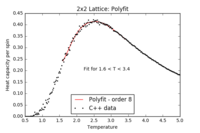
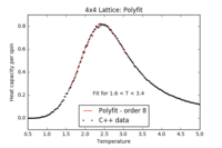
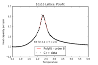
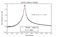
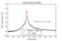
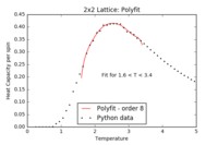
For the remainder of the report, a polyfit order of 8 has been chosen: high enough to obtain a good fit, but sufficiently low to avoid poorly optimised high-order term fits.

TASK: find the temperature at which the maximum in C occurs for each datafile that you were given. Make a text file containing two colums: the lattice side length (2,4,8, etc.), and the temperature at which C is a maximum. This is your estimate of $T_{C}$ for that side length. Make a plot that uses the scaling relation given above to determine $T_{C, \infty}$ . By doing a little research online, you should be able to find the theoretical exact Curie temperature for the infinite 2D Ising lattice. How does your value compare to this? Are you surprised by how good/bad the agreement is? Attach a PNG of this final graph to your report, and discuss briefly what you think the major sources of error are in your estimate.

2x2 Polyfit	4x4 Polyfit	8x8 Polyfit	16x16 Polyfit	32x32 Polyfit	64x64 Polyfit

T_{C, L} = \frac{A}{L} + T_{C, \infty}

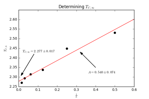
A plot of $T_{C, L}$ against $\frac{1}{L}$ yields a straight line, with intercept $T_{C, \infty}$ and gradient $A$ (a constant). Fitting the C++ data resulted in a value for $T_{C, \infty} = 2.277 \pm 0.017 \frac{J}{k_{B}}$ , with the uncertainty calculated from the error in the linear fit. This is in good agreement with the reference value^[1] of $T_{C, \infty} \approx 2.269 \frac{J}{k_{B}}$ . The main source of error is the fitting of the straight line, which is quantifiable and represents a 1% uncertainty. There is also an uncertainty in the extraction of $T_{C, L}$ values from the polynomial fitting of the peaks in each heat capacity plot, as the fits are not exact. The simulations themselves also introduce an uncertainty: for example, if the lattice did not equilibrate within the limit of the number of simulation steps.

However, this experiment has reproduced the theoretical value within the error of the straight line fit, demonstrating the power of the Monte Carlo methods used.

Locating the Curie temperature - Python data

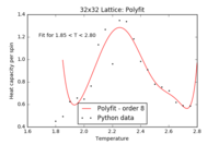
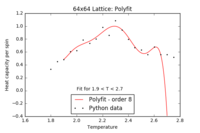
Below are the fitted functions for the Python heat capacity data. For the 16x16, 32x32 and 64x64 lattices, the averaged data points over 10 repeats were used (see above).

2x2 Polyfit	4x4 Polyfit	8x8 Polyfit	16x16 Polyfit	32x32 Polyfit	64x64 Polyfit

Compiling this data to plot the straight line, as outlined previously, yielded very similar results to the C++ data:

There is a larger uncertainty in the fitting of the straight line but the resulting curie temperature, $T_{C, \infty} = 2.28 \pm 0.03 \frac{J}{k_{B}}$ , is nearly identical to the result from the C++ data and is in good agreement with the reference value^[1]. Due to the noise in the heat capacity plots in the critical temperature region, the polynomial fits of the peaks were not as convincing as the fits for the C++ data. The $T_{C, L}$ values that were subsequently extracted from these polynomial fits were shifted from the C++ data, resulting in the greater spread of data points in the straight line plot above. Furthermore, there are contributing errors from the simulations themselves - for example, the lattice not reaching equilibrium or getting stuck in a local minimum (the 'clumping' effect discussed earlier) affecting the heat capacity.

References

1 B. Liu, M. Gitterman, American Journal of Physics, 71, 806 (2003), pp. 1-4

2 R. Fitzpatrick, 2006, The Ising Model, Computational Physics, retrieved from http://farside.ph.utexas.edu/teaching/329/lectures/node110.html in November 2017.

3 P. Atkins and J. de Paula, Atkins' Physical Chemistry, Oxford University Press, UK, 8th edn, 2006, pp. 564-573