Rep:Third year CMP compulsory experimentRG1712

Introduction to the Ising Model

The Ising Model

TASK 1: (i) Show that the lowest possible energy for the Ising model is $E = - D N J$ , where $D$ is the number of dimensions and $N$ is the total number of spins. (ii) What is the multiplicity of this state? (iii) Calculate its entropy.

(i) In the absence of a magnetic field, the interaction energy of the Ising lattice may be represented as follows, $- \frac{1}{2} J \sum_{i}^{N} \sum_{j \in n e i g h b o u r s (i)} s_{i} s_{j}$ , where J is the exchange constant. A positive value of the exchange constant J indicates a favourable exchange energy for a spin system in which the spins are aligned parallel. Under the assumptions of the model, the sole contributions to the total energy arise from interactions between adjacent atoms in the lattice. Given these conditions, the lowest energy configuration for the 1D case corresponds to a linear chain of atoms with parallel spins. Each atom in this chain possesses two neighbours and thus will contribute $- 2 J$ to the total energy. A similar argument yields contributions of $- 4 J$ and $- 6 J$ per spin for the 2D and 3D lattices respectively. Hence it may be inferred that the contribution per spin in a D dimensional system will be $- 2 D J$ . When the pre-factor of $\frac{1}{2}$ is accounted for and the individual contributions from the spins summed, a generalised result of $- D N J$ is obtained for the lowest possible energy.

(ii) In contrast to the spin multiplicity known to chemists, the term "multiplicity" in statistical mechanics refers to a system's available microstates. In the case of the lowest possible energy lattice there are 2 microstates, one in which all of the spins pointe up (+1) and one in which all of the spins point down (-1). As such, one may say that the multiplicity of the system is 2.

(iii) The entropy of the system may be computed using Boltzmann's equation, $S = K b l n (W)$ , where Kb is Boltzmann's constant and W is the number of microstates. Taking Kb to be 1.381 x 10^-23 JK^-1 and W to be 2, the entropy is calculated to be 9.572 x 10^-24 JK^-1.

Phase Transitions

TASK 2: Imagine that the system is in the lowest energy configuration. To move to a different state, one of the spins must spontaneously change direction ("flip"). (i) What is the change in energy if this happens ( $D = 3, N = 1000$ )? (ii) How much entropy does the system gain by doing so?

(i) As mentioned in the answer to task 1, the contribution to the total energy for a single spin in a 3D lattice, with only spin-parallel neighbours, is $- 6 J$ . Flipping this single spin would serve to create an unfavourable interaction with its six neighbours. Hence the new contribution for this spin would be $+ 6 J$ . The difference between these two values gives the net energy change of $+ 12 J$ . In other words the total energy of the state with a single flipped spin would be raised to $- 2988 J$ .

(ii) There are 1000 atoms in the lattice. Assuming that each of these atoms is equally likely to be the flipped spin there are 1000 microstates. Again this number must be corrected by a factor of 2 due to the equivalence of the up and down configurations yielding 2000 microstates. In other words 999 spins may be up while 1 is down or 1 may be up while 999 are down. The entropy may be computed as previously described using the Boltzmann equation S = Kbln(2000) giving a value of 1.050 x 10-22 JK^-1. The difference in entropy between the states represents the entropy gained on flipping. 1.050 x 10^-22 JK^-1 - 9.572 x 10^-24 JK^-1 = 9.540 x 10^-23 JK^-1.

TASK 3: (i) Calculate the magnetisation of the 1D and 2D lattices in figure 1. (ii) What magnetisation would you expect to observe for an Ising lattice with $D = 3, N = 1000$ at absolute zero?

(i) The total magnetisation is given by $M = \sum_{i} s_{i}$ . In the 1D case 3 of the spins have a value of +1 while two of the spins have a value of -1. Hence summing these values one obtains a total magnetisation of +1. Similarly in the 2D case, 13 spins have a value of +1 while 12 spins have a value of -1. Again, summing these values yields a total magnetisation of +1.

(ii) At absolute zero there is no thermal energy present in the system and hence spin-flipping processes will not be observed. As such, the spins will be aligned parallel yielding magnetisation values of either +1000 or -1000 dependent on whether the spins are pointing upwards or downwards.

Calculating The Energy and Magnetisation

Modifying The Files

TASK 4: complete the functions energy() and magnetisation(), which should return the energy of the lattice and the total magnetisation, respectively. In the energy() function you may assume that $J = 1.0$ at all times (in fact, we are working in reduced units in which $J = k_{B}$ , but there will be more information about this in later sections). Do not worry about the efficiency of the code at the moment — we will address the speed in a later part of the experiment.

The lattice is represented as type numpy.ndarray and may be N dimensional. The elements of the lattice are also of type numpy.ndarray and will be the individual rows of the lattice. Each row consists of a sequence of spins. Each spin may have a value of either 1 or -1. The energy is given by spin-spin interactions and will take values of +1 or -1 (from the product of the spin values) depending on whether two spins have the same value or not. As the lattice is two-dimensional, each spin will have 4 neighbours and hence the spin's contribution to the total energy will take into account these 4 interactions. A problem would arise if each spin in the lattice was iterated over and these 4 interactions calculated in each case; the interactions would be over counted. Fortunately there is a simple solution to this problem. An iteration is implemented whereby each spin in each row is accessed and its interactions with just two spins are considered. These spins will lie to the right (next spin in the row) and immediately beneath it (spin with the same spin index but in the next row index of the lattice). "There are two cases in which accounting for the 'below and to the right' interactions will require some extra thought. These cases occur on separate levels. In the first instance, there will be a problem when the last row of the lattice is reached. Due to the periodic boundary conditions, these spins may be referred to the first row of the lattice. The spins of the first row may then be considered to be lying below the spins of the last row. In the second instance, the last spin of every row will not have a neighbour to its right. Again due to the periodic boundary conditions, the last spin in each row may be referred back to the first spin in the same row. Thus exceptions must be tested for at the level of first the lattice indexing and then the row indexing.



def energy(self):

   "Return the total energy of the current lattice configuration." 

   # The equation used to calculate the energy of a configuration is given by -0.5J times the sum over the products of nearest neighbour's spins. 
   # https://wiki.ch.ic.ac.uk/wiki/index.php?title=Third_year_CMP_compulsory_experiment/Introduction_to_the_Ising_model
   # Iterate over each spin in the lattice once and note of its contribution to the total lattice energy

    energy = 0

    row_counter = 0

    for row in self.lattice:

       if row_counter == len(self.lattice) - 1:

          #Last row in lattice has been reached
          #No row below this one and so it is necessary to refer it back to the first row
          #The spin_counter variable is set to 0 before we access the the first spin in the row

          spin_counter = 0

          #running over spins in a given row

          for spin in row:

             if spin_counter == len(row) - 1:
       
                #Last spin in row has been reached
                #As this is the last row, the spin element beneath the spin being accessed may be found in the first row
                #This trick overcomes the boundary conditions imposed by a finite lattice


                energy += ((spin*(row[0])) + (spin*(self.lattice[0][spin_counter])))

                #running value of energy updated

             else:

                #spin is not last in row

                energy += ((spin*(row[spin_counter + 1])) + (spin*(self.lattice[0][spin_counter])))

                spin_counter += 1

       else:

          #Row is not the last row in the lattice
          #Procedure similar to above


          spin_counter = 0

          for spin in row:

             if spin_counter == len(row) -1:

                energy += ((spin*(row[0])) + (spin*(self.lattice[row_counter + 1][spin_counter])))

             else:

                energy += ((spin*(row[spin_counter + 1])) + (spin*(self.lattice[row_counter + 1][spin_counter])))

                spin_counter += 1


          row_counter += 1

          #next row 

    return energy


def magnetisation(self):

    "Return the total magnetisation (in reduced units) of the current lattice configuration."

    #Each atom in the lattice is accessed and its spin value is added to the running total
    #https://wiki.ch.ic.ac.uk/wiki/index.php?title=Third_year_CMP_compulsory_experiment/Introduction_to_the_Ising_model

    magnetisation = 0.0
    
    #Running total initialised

    for row in self.lattice:

       for spin in row:

          magnetisation += spin

    return magnetisation

Testing The Files

TASK 5: Run the ILcheck.py script from the IPython Qt console using the command

%run ILcheck.py

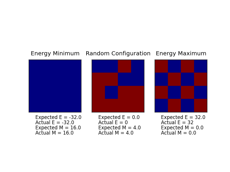
The displayed window has a series of control buttons in the bottom left, one of which will allow you to export the figure as a PNG image. Save an image of the ILcheck.py output, and include it in your report.

The expected values for the energy and magnetisation of the test cases are produced.

Introduction to The Monte Carlo Simulation

Average Energy and Magnetisation

TASK 6: (i) How many configurations are available to a system with 100 spins? To evaluate these expressions, we have to calculate the energy and magnetisation for each of these configurations, then perform the sum. Let's be very, very, generous, and say that we can analyse $1 \times 1 0^{9}$ configurations per second with our computer. (ii) How long will it take to evaluate a single value of ${⟨ M ⟩}_{T}$ ?

(i) The number of configurations available to a system with N spins may be generalised as $W = n^{N}$ where W is the number of configurations and n is the number of states available to a single spin. In this case the spins may point either upwards or downwards and hence $n = 1$ . For 100 spins W has a value of $2^{100}$ or in other words there are $1.268 \times 1 0^{30}$ configurations available to the system.

(ii) Given a processing speed of $1 \times 1 0^{9}$ configurations per second, it would take $4 \times 1 0^{13}$ years to compute a single value for the average magnetisation at a single temperature!

Importance Sampling

Modifying IsingLattice.py

TASK 7: Implement a single cycle of the above algorithm in the montecarlocycle(T) function. This function should return the energy of your lattice and the magnetisation at the end of the cycle. You may assume that the energy returned by your energy() function is in units of $k_{B}$ ! Complete the statistics() function. This should return the following quantities whenever it is called: $< E >, < E^{2} >, < M >, < M^{2} >$ , and the number of Monte Carlo steps that have elapsed.

It is computationally impossible to include every configuration for the purposes of determining average values for the energy or magnetisation of a system. As such a Metropolis Monte Carlo (MMC) algorithm is used in order to effect importance sampling on the configurations. The 'importance' of a configuration is given by its Boltzmann factor. A spin is flipped in the input lattice. The energy of this new configuration is compared to the original lattice. If the energy of the new lattice is lower than that of the original lattice, the configuration is accepted. The energy and magnetisation values of the new lattice are then added to the running sum of the sampled configuration energies and magnetisations respectively. If the energy of the new lattice is higher than that of the original lattice, a random number is generated. If the random number is less than the new configuration's Boltzmann factor, the configuration is accepted as above. If the random number is greater than the new configuration's Boltzmann factor, the configuration is rejected and the old configuration is retained. The vales for the energy (in reduced units of Kb) and magnetisation of the accepted lattice are returned.


def montecarlostep(self, T):

   "Return the energy in reduced units of Kb and magnetisation (unitless) values of the accepted configuration."
    #This method implements a single step of the MMC algorithm http://web.chem.ucsb.edu/~kalju/MonteCarlo_3.html
    #Flip a spin in the lattice self
    #Accept the new configuration if the energy is lower than the initial configuration
    #If the energy is higher, acceptance will depend on the configuration's Boltzmann factor and on the random number generator

    random_i = np.random.choice(range(0, self.n_rows))

    random_j = np.random.choice(range(0, self.n_cols))

    #Random spin to be flipped
    #A random_number variable is defined for use later on, when a random number will need to be generated and compared to the 
    Boltzmann factor of a configuration

    random_number = np.random.random()

    #Two variables, E_Orig and M_Orig are created to store the values of the original input lattice's energy and magnetisation

    E_Orig = self.energy()

    M_Orig = self.magnetisation()

    self.lattice[random_i][random_j] *= -1

    #Random spin flipped
    #Three variables are created, two to store the values of the new lattice's energy and magnetisation and a 
    third to store the energy difference between configurations."

    E_Flip = self.energy()

    M_Flip = self.magnetisation()

    Energy_Diff = E_Flip - E_Orig

    #A test is carried out to determine whether or not the new configuration is lower in 
    energy relative to the original configuration

    if Energy_Diff <= 0:

       #Configuration accepted
       #Running sums updated

       energy = E_Flip

       magnetisation = M_Flip

       self.E += energy

       self.M += magnetisation

       self.E2 += energy**2

       self.M2 += magnetisation**2

    elif Energy_Diff > 0:

      #If the new configuration is higher in energy a random number test is carried out

      if random_number <= np.exp((-1*Energy_Diff)/T):

          #If the randomly generated number if smaller than the configuration's Boltzmann factor 
          the configuration is accepted and the algorithm proceeds as in the accepted case above

          energy = E_Flip
          magnetisation = M_Flip
          self.E += energy
          self.M += magnetisation
          self.E2 += energy**2
          self.M2 += magnetisation**2

       elif random_number > np.exp((-1*Energy_Diff)/T):

          #If the randomly generated number is larger than the configuration's Boltzmann factor, 
          the configuration is rejected
          #The values of the energy and magnetisation values returned are those of the original lattice
          #The configuration is reverted to that of the original lattice

          energy = E_Orig
          magnetisation = M_Orig
          self.E += energy
          self.M += magnetisation
          self.E2 += energy**2
          self.M2 += magnetisation**2
          self.lattice[random_i][random_j] *= -1

   "The cycle count is increased by one on completion of the step."

    self.n_cycles += 1

    return energy, magnetisation

def statistics(self):

   "Return average energy, square energy, magnetisation and square 
    magnetisation of the sampled configurations as well as number of completed cycles."

   #Averaged values are computed by dividing the running sum by the 
    number of cycles for each parameter. Again aveE in reduced units of Kb."

    aveE = self.E/self.n_cycles
    aveE2 = self.E2/self.n_cycles
    aveM = self.M/self.n_cycles
    aveM2 = self.M2/self.n_cycles

    return aveE, aveE2, aveM, aveM2, self.n_cycles

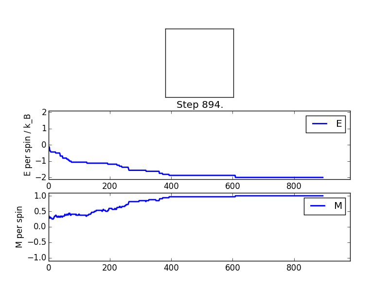
TASK 8: (i) If $T < T_{C}$ , do you expect a spontaneous magnetisation (i.e. do you expect $⟨ M ⟩ \neq 0$ )? (ii) When the state of the simulation appears to stop changing (when you have reached an equilibrium state), use the controls to export the output to PNG and attach this to your report. You should also include the output from your statistics() function.

(i) Below the Curie Temperature spontaneous magnetisation is to be expected. In this case the absolute value of the average magnetisation will be non-zero. At 0 temperature $⟨ M ⟩$ will rise to a figure whose absolute value is equatable to the number of spins in the system. In general as temperature increases $⟨ M ⟩$ will decrease, reaching a value of 0 above the Curie Temperature.

(ii) The output from the statistics function is provided in table 1. One may see from the figures that the value of the average energy per spin converges to a value of -2 and similarly that the value of the average magnetisation per spin converges to a value of +1 for this particular Monte Carlo simulation. It should be noted that the values output by the statistics function are sensitive to the fluctuations in these parameters experienced when moving towards equilibrium. As such the results will not be in excellent agreement with the converged values.

Table 1. Averaged Quantities output by the Statistics Function.
Energy	-1.28713002114
Square Energy	2.01484044662
Magnetisation	0.672106236786
Square Magnetisation	0.577036948335
Number of Cycles	473

Accelerating The Code

TASK 9: Use the script ILtimetrial.py to record how long your current version of IsingLattice.py takes to perform 2000 Monte Carlo steps. This will vary, depending on what else the computer happens to be doing, so perform repeats and report the error in your average!

Table 2. Duration of trials performing 2000 Monte Carlo steps using the Unaccelerated Code.
Trial	Duration (seconds)
1	2.192724657026057
2	2.2323801089149224
3	2.2153646047932583
4	2.2407804009887524
5	2.2363479783788076
6	2.2163924173093896s
7	2.2227446306983616
8	2.2291792502009606
9	2.2231186276755928
10	2.23662296727813
Standard Error	0.004242866

TASK 10: Look at the documentation for the NumPy sum function. You should be able to modify your magnetisation() function so that it uses this to evaluate M. The energy is a little trickier. Familiarise yourself with the NumPy roll and multiply functions, and use these to replace your energy double loop (you will need to call roll and multiply twice!).

   

def energy(self):

   "Return energy of lattice in reduced units of Kb."

   #Function making use of matrix linear algebra

    energy = 0

    energy -= ((np.sum(np.multiply(self.lattice, np.roll(self.lattice, 1, axis = 0)))) + (np.sum(np.multiply(self.lattice, 
    np.roll(self.lattice, 1, axis =   1)))))

    return energy

def magnetisation(self):

   "Return net magnetisation of lattice (unitless)."

    magnetisation = np.sum(self.lattice)

    return magnetisation

TASK 11: Use the script ILtimetrial.py to record how long your new version of IsingLattice.py takes to perform 2000 Monte Carlo steps. This will vary, depending on what else the computer happens to be doing, so perform repeats and report the error in your average!

Table 3. Duration of trials performing 2000 Monte Carlo steps using the Accelerated Code.
Trial	Duration (seconds)
1	0.14375671058860462
2	0.14221061493390152
3	0.1363163139048993
4	0.13915434423597617
5	0.1400740930575921
6	0.1415220861972557
7	0.14384273894938815
8	0.13966206248915114
9	0.14755101406353788
10	0.1476786982602789
Standard Error	0.001091238

This difference in speed is not due to improved time complexity on the part of the new algorithm. Instead the reason lies in the fact that numpy functions are based in C++, a language with better memory cache properties relative to Python. The difference in speed reflects the difference between a compiled language (C++) and an interpreted one (Python).

The Effect of Temperature

Correcting The Averaging Code

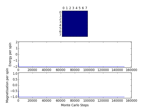
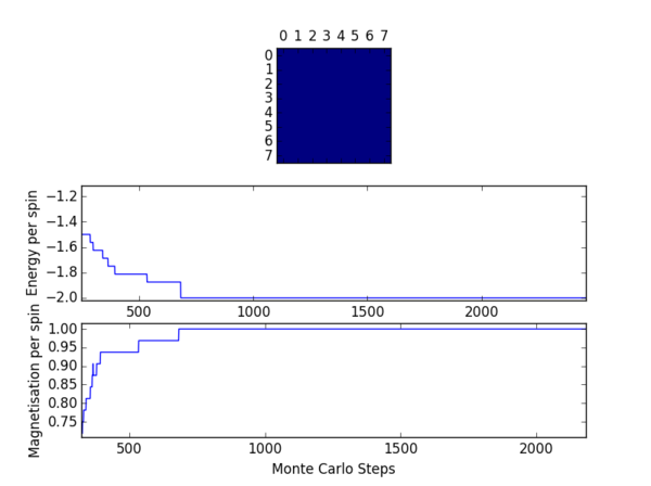
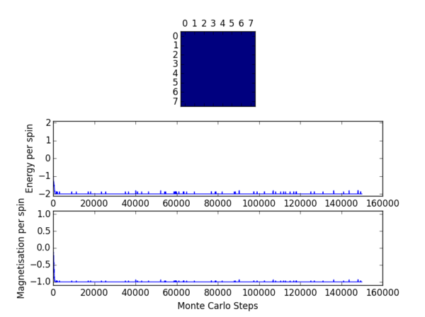
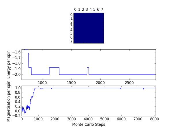
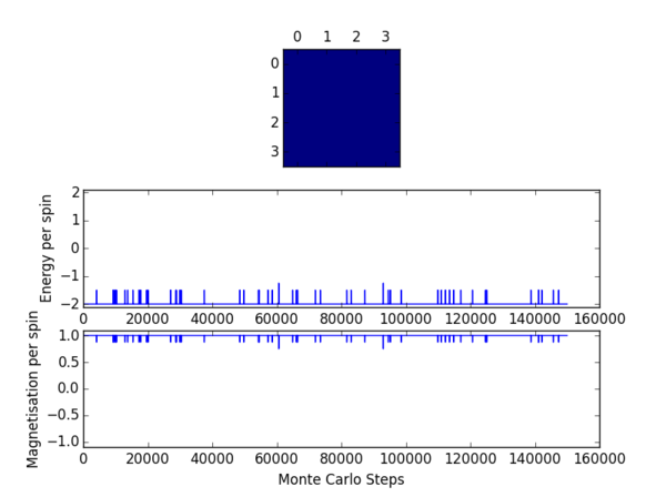
TASK 12: The script ILfinalframe.py runs for a given number of cycles at a given temperature, then plots a depiction of the final lattice state as well as graphs of the energy and magnetisation as a function of cycle number. This is much quicker than animating every frame! Experiment with different temperature and lattice sizes. (i) How many cycles are typically needed for the system to go from its random starting position to the equilibrium state? Modify your statistics() and montecarlostep() functions so that the first N cycles of the simulation are ignored when calculating the averages. You should state in your report what period you chose to ignore, and include graphs from ILfinalframe.py to illustrate your motivation in choosing this figure.

The code for the omission of the cycles performed while the system is in the process of reaching equilibrium is provided below.


def montecarlostep(self, T):

   "Return the energy in reduced units of Kb and magnetisation (unitless) values of the accepted configuration."

   random_i = np.random.choice(range(0, self.n_rows))

   random_j = np.random.choice(range(0, self.n_cols))

   random_number = np.random.random()

   E_Orig = self.energy()

   M_Orig = self.magnetisation()

   self.lattice[random_i][random_j] *= -1

   E_Flip = self.energy()

   M_Flip = self.magnetisation()

   Energy_Diff = E_Flip - E_Orig

   if Energy_Diff <= 0:

      energy = E_Flip

      magnetisation = M_Flip

   elif Energy_Diff > 0:

      if random_number <= np.exp((-1*Energy_Diff)/T):

         energy = E_Flip

         magnetisation = M_Flip

      elif random_number > np.exp((-1*Energy_Diff)/T):

         energy = E_Orig

         magnetisation = M_Orig

         self.lattice[random_i][random_j] *= -1

   if self.n_cycles >= 500:

      #Only update running sums when the number of cycles has reached a certain value

      self.E += energy

      self.M += magnetisation

      self.E2 += energy**2

      self.M2 += magnetisation**2

   self.n_cycles += 1

   return energy, magnetisation

def statistics(self):

   #Subtract the number of cycles omitted from the cycle counter

   aveE = self.E/(self.n_cycles - 500)
   aveE2 = self.E2/(self.n_cycles - 500)
   aveM = self.M/(self.n_cycles - 500)
   aveM2 = self.M2/(self.n_cycles - 500)

   return aveE, aveE2, aveM, aveM2, self.n_cycles

The effect of temperature on the number of steps required to reach equilibrium may be observed from the figures in table 4. As the temperature is increased a greater number of cycles is required before the system can equilibrate. Higher temperatures favour a more entropic configuration. As such the driving force for obtaining an enthalpically favourable configuration is diminished somewhat, resulting in a longer time period before equilibrium may be attained. One should note that at a temperature of 2.5 (reduced units) the system will not equilibrate at all.

Table 4. The Number of Steps Required to Reach Equilibrium - The Effect of Temperature.
Temperature (Reduced Units)	Close-up View	Number of Cycles Necessary to Omit
0.1		800
0.5		1200
1.0		1400
1.5		2000
2.0		2000
2.5	Behaviour evident from first graph	Does not Equilibrate

The effects of system size were also investigated. In general a greater number of spins will necessitate a longer induction period before equilibrium is reached. One would expect this intuitively since it will be much more difficult to align a larger number of spins preferentially. The effects of lattice size were the primary determinant for the number of cycles to be omitted in subsequent exercises.

Table 5. The Number of Steps Required to Reach Equilibrium - The Effect of Lattice Size.
Lattice Size	Graph of Energy/Magnetisation per Spin versus Number of Steps	Number of Cycles Necessary to Omit
2x2		100
4x4		200
8x8		2500
16x16		7000
32x32		150000

Running over a Range of Temperatures

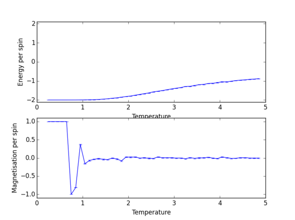
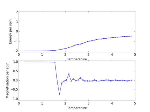
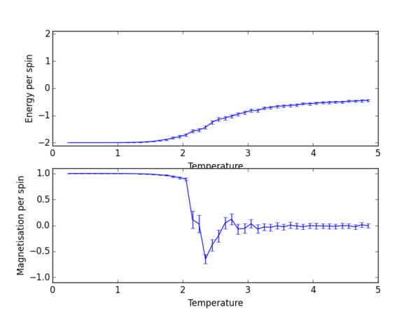
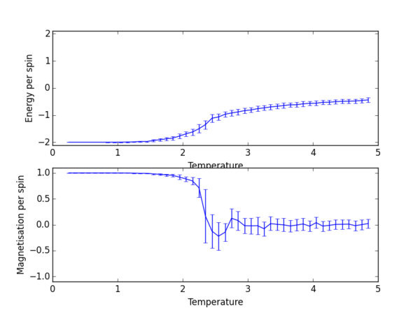
TASK 13: Use ILtemperaturerange.py to plot the average energy and magnetisation for each temperature, with error bars, for an $8 \times 8$ lattice. Use your initution and results from the script ILfinalframe.py to estimate how many cycles each simulation should be. The temperature range 0.25 to 5.0 is sufficient. Use as many temperature points as you feel necessary to illustrate the trend, but do not use a temperature spacing larger than 0.5. T NumPy function savetxt() stores your array of output data on disk — you will need it later. Save the file as 8x8.dat so that you know which lattice size it came from.


from IsingLattice import *

from matplotlib import pylab as pl

import numpy as np

n_rows = 2

n_cols = 2

il = IsingLattice(n_rows, n_cols)

il.lattice = np.ones((n_rows, n_cols))

spins = n_rows*n_cols

runtime = 100000

times = range(runtime)

temps = np.arange(0.25, 4.95, 0.1)

#np.arange(starting temperature, finishing temperature, temperature step)

energies = []
magnetisations = []
energysq = []
magnetisationsq = []

#Lists created to store error values

energyer = []
magnetisationer = []

for t in temps:

   for i in times:

      if i % 100 == 0:

         print(t, i)

      energy, magnetisation = il.montecarlostep(t)

   aveE, aveE2, aveM, aveM2, n_cycles = il.statistics()

   energies.append(aveE)

   energysq.append(aveE2)

   magnetisations.append(aveM)

   magnetisationsq.append(aveM2)

   #Standard errors given by standard deviation divided by the square root of the number of runs

   energyer.append(np.sqrt(aveE2 - (aveE**2))/(np.sqrt(n_cycles)))

   magnetisationer.append(np.sqrt(aveM2 - (aveM**2))/(np.sqrt(n_cycles)))

   #reset the IL object for the next cycle

   il.E = 0.0

   il.E2 = 0.0

   il.M = 0.0

   il.M2 = 0.0

   il.n_cycles = 0

fig = pl.figure()

enerax = fig.add_subplot(2,1,1)

enerax.set_ylabel("Energy per spin")

enerax.set_xlabel("Temperature")

enerax.set_ylim([-2.1, 2.1])

magax = fig.add_subplot(2,1,2)

magax.set_ylabel("Magnetisation per spin")

magax.set_xlabel("Temperature")

magax.set_ylim([-1.1, 1.1])

# http://matplotlib.org/api/pyplot_api.html - documentation for errorbar method

enerax.errorbar(temps, np.array(energies)/spins, yerr = energyer)

magax.errorbar(temps, np.array(magnetisations)/spins, yerr = magnetisationer)

pl.show()

final_data = np.column_stack((temps, energies, energysq, magnetisations, magnetisationsq))

np.savetxt("lattice_2x2_RG1712.dat", final_data)

Table 6. Energy/Magnetisation per Spin vs. Temperature - The Effect of Lattice Size.
Lattice Size	Number of Cycles Omitted	Runtime
2x2	500	100000
4x4	500	100000
8x8	2500	100000
16x16	7000	100000
32x32	30000	400000

In the case of the 32x32 lattice 30000 steps were omitted as opposed to 150000 in the process of trying to debug the code responsible for omitting N cycles. Serendipitously, the omission of 30000 steps produced a reasonable graph and so was kept.

The Effect of System Size

Scaling The System Size

TASK 14: Repeat the final task of the previous section for the following lattice sizes: 2x2, 4x4, 8x8, 16x16, 32x32. Make sure that you name each datafile that your produce after the corresponding lattice size! Write a Python script to make a plot showing the energy per spin versus temperature for each of your lattice sizes. Hint: the NumPy loadtxt function is the reverse of the savetxt function, and can be used to read your previously saved files into the script. Repeat this for the magnetisation. As before, use the plot controls to save your a PNG image of your plot and attach this to the report. (i) How big a lattice do you think is big enough to capture the long range fluctuations?

(i) The easiest comparison can be made if the results of all lattice sizes are plotted on the same graph.


from matplotlib import pylab as pl

import numpy as np

fig = pl.figure()

enerax = fig.add_subplot(2,1,1)

enerax.set_ylabel("Energy per spin")

enerax.set_xlabel("Temperature")

enerax.set_xlim([0, 5])

magax = fig.add_subplot(2,1,2)

magax.set_ylabel("Magnetisation per spin")

magax.set_xlabel("Temperature")

magax.set_xlim([0,5])

magax.set_ylim([-1.1, 1.1])

lattice_2x2 = np.loadtxt("lattice_2x2_RG1712.dat")

lattice_4x4 = np.loadtxt("lattice_4x4_RG1712.dat")

lattice_8x8 = np.loadtxt("lattice_8x8_RG1712.dat")

lattice_16x16 = np.loadtxt("lattice_16x16_RG1712.dat")

lattice_32x32 = np.loadtxt("lattice_32x32_RG1712.dat")

Collection = [lattice_2x2, lattice_4x4, lattice_8x8, lattice_16x16, lattice_32x32]

#Make a list of the data pertaining to the different lattice sizes

size = 1

for lattice in Collection:

   #Loop over the list, plotting the data from each file

   temps = lattice[:,0]

   energies = lattice[:,1]

   energysq = lattice[:,2]

   magnetisations = lattice[:,3]

   magnetisationssq = lattice[:,4]

   spins = np.square(size*2)

   enerax.plot(temps, np.array(energies)/spins, label = str(size*2) + "x" + str(size*2))

   enerax.legend(loc = 0, fontsize = 'x-small')

   magax.plot(temps, np.array(magnetisations)/spins, label = str(size*2) + "x" + str(size*2))

   magax.legend(loc = 1, fontsize = 'x-small')

   size *= 2

pl.show()

(i) The 8x8 lattice is probably good enough to capture long range fluctuations. By eye, from the graph, one can judge that there is little improvement to be obtained on doubling the lattice size to 16x16. Hence 8x8 probably represents the best balance between accuracy and computational expense.

Determining The Heat Capacity

Calculating The Heat Capacity

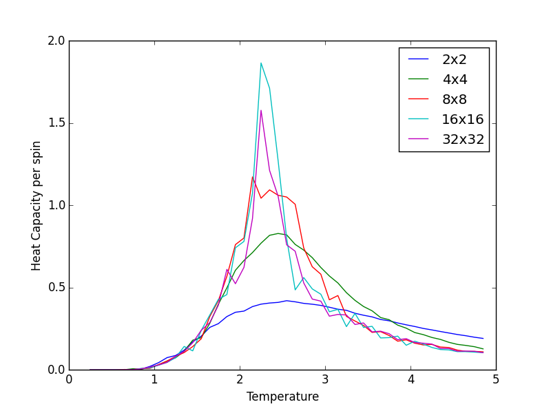
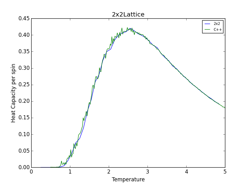
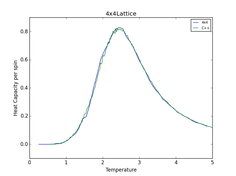
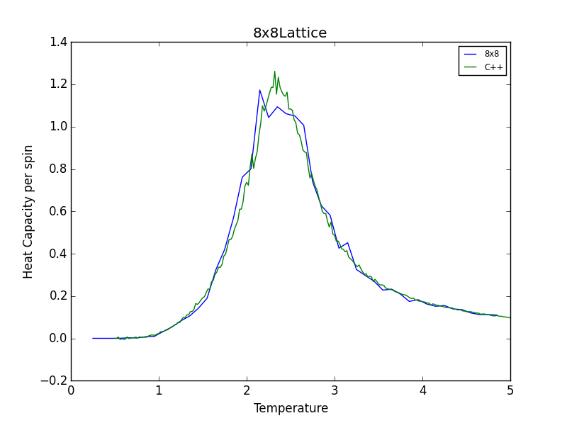
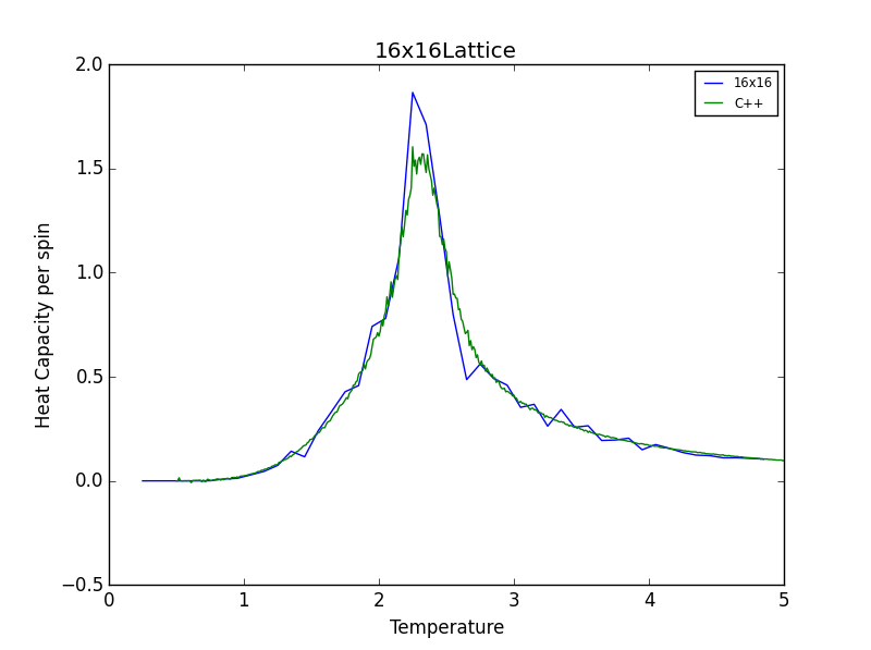
TASK 15: Write a Python script to make a plot showing the heat capacity versus temperature for each of your lattice sizes from the previous section. You may need to do some research to recall the connection between the variance of a variable, $V a r [X]$ , the mean of its square $⟨ X^{2} ⟩$ , and its squared mean ${⟨ X ⟩}^{2}$ . You may find that the data around the peak is very noisy — this is normal, and is a result of being in the critical region. As before, use the plot controls to save your a PNG image of your plot and attach this to the report.

The Heat Capacity is given by ( $⟨ E^{2} ⟩$ - ${⟨ E ⟩}^{2}$ )/ $k_{B} T^{2}$ where the numerator represents the variance of the variable 'energy'.


from matplotlib import pylab as pl

import numpy as np

fig = pl.figure()

HCax = fig.add_subplot(1,1,1)

HCax.set_ylabel("Heat Capacity per spin")

HCax.set_xlabel("Temperature")

lattice_2x2 = np.loadtxt("lattice_2x2_RG1712.dat")

lattice_4x4 = np.loadtxt("lattice_4x4_RG1712.dat")

lattice_8x8 = np.loadtxt("lattice_8x8_RG1712.dat")

lattice_16x16 = np.loadtxt("lattice_16x16_RG1712.dat")

lattice_32x32 = np.loadtxt("lattice_32x32_RG1712.dat")

Collection = [lattice_2x2, lattice_4x4, lattice_8x8, lattice_16x16, lattice_32x32]

size = 2

for lattice in Collection:

   temps = lattice[:,0]

   energies = lattice[:,1]

   energysq = lattice[:,2]

   spins = np.square(size)

   variance = (energysq - np.square(energies))/(spins)

   #variance divided by the number of spins in order to give the heat capacity per spin in the plot

   HCax.plot(temps, (variance)/(np.square(temps)), label = str(size) + "x" + str(size))

   HCax.legend(loc = 0)

   size *= 2

pl.show()

Locating The Curie Temperature

TASK 16: A C++ program has been used to run some much longer simulations than would be possible on the college computers in Python. You can view its source code here if you are interested. Each file contains six columns: $T, E, E^{2}, M, M^{2}, C$ (the final five quantities are per spin), and you can read them with the NumPy loadtxt function as before. For each lattice size, plot the C++ data against your data. For one lattice size, save a PNG of this comparison and add it to your report — add a legend to the graph to label which is which. To do this, you will need to pass the label="..." keyword to the plot function, then call the legend() function of the axis object (documentation here).


from matplotlib import pylab as pl

import numpy as np

#Load Python and C++ data files and plot both on the same graph

lattice_2x2 = np.loadtxt("lattice_2x2_RG1712.dat")

lattice_4x4 = np.loadtxt("lattice_4x4_RG1712.dat")

lattice_8x8 = np.loadtxt("lattice_8x8_RG1712.dat")

lattice_16x16 = np.loadtxt("lattice_16x16_RG1712.dat")

lattice_32x32 = np.loadtxt("lattice_32x32_RG1712.dat")

lattice_2x2_C = np.loadtxt("2x2.dat")

lattice_4x4_C = np.loadtxt("4x4.dat")

lattice_8x8_C = np.loadtxt("8x8.dat")

lattice_16x16_C = np.loadtxt("16x16.dat")

lattice_32x32_C = np.loadtxt("32x32.dat")

Collection = [lattice_2x2, lattice_4x4, lattice_8x8, lattice_16x16, lattice_32x32]

Collection_C = [lattice_2x2_C, lattice_4x4_C, lattice_8x8_C, lattice_16x16_C, lattice_32x32_C]

size = 1

i = 0

for lattice in Collection:

   fig = pl.figure()

   pl.title(str(size*2) + "x" + str(size*2) + "Lattice")

   HCax = fig.add_subplot(1,1,1)

   HCax.set_ylabel("Heat Capacity per spin")

   HCax.set_xlabel("Temperature")

   temps = lattice[:,0]

   energies = lattice[:,1]

   energysq = lattice[:,2]

   spins = np.square(size*2)

   variance = (energysq - np.square(energies))/(spins)

   HCax.plot(temps, variance/np.square(temps), label = str(size*2) + "x" + str(size*2))

   HCax.legend(loc = 2)

   temps = Collection_C[i][:,0]

   HCs = Collection_C[i][:,5]

   HCax.plot(temps, HCs, label = "C++")

   HCax.legend(loc = 0, fontsize = 'x-small')

   pl.show()

   i += 1

   size *= 2

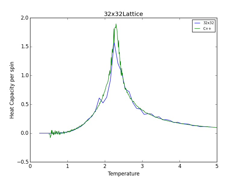
The figures below show good agreement between the Heat Capacity vs. Temperature plots produced. Deviation seems to become more pronounced as lattice size increases.

Polynomial Fitting

TASK 17: write a script to read the data from a particular file, and plot C vs T, as well as a fitted polynomial. Try changing the degree of the polynomial to improve the fit — in general, it might be difficult to get a good fit! Attach a PNG of an example fit to your report.


from matplotlib import pylab as pl

import numpy as np

#Fit polynomials of increasing order to the same data

fig = pl.figure()

pl.title("A Comparison of Polynomial Fits to the Data")

HCax = fig.add_subplot(1,1,1)

HCax.set_ylabel("Heat Capacity per spin")

HCax.set_xlabel("Temperature")

degree = 442

#degree of polynomial at which to stop specified here

data = np.loadtxt("64x64.dat")

T = data[:,0] #get the first column

C = data[:,5] # get the fifth column

HCax.plot(T,C, "yo",label = "Data Points")

while degree <= 442:

   #specify degree of polynomial at which to stop

   #first we fit the polynomial to the data

   fit = np.polyfit(T, C, degree) # fit the order polynomial given by variable degree.

   #now we generate interpolated values of the fitted polynomial over the range of our function

   Tmin = np.min(T)

   Tmax = np.max(T)

   T_range = np.linspace(Tmin, Tmax, 1000) #generate 1000 evenly spaced points between T_min and T_max

   fitted_C_values = np.polyval(fit, T_range) # use the fit object to generate the corresponding values of C

   HCax.plot(T_range, fitted_C_values, label = str(degree) + "nd" + " " + "order" + " " + "fit")

   HCax.legend(loc = 0, fontsize = 'x-small')

   degree *= 2

   #degree of polynomial increased by a factor of 2 if limit of while loop has not yet been reached

pl.show()

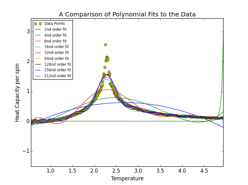
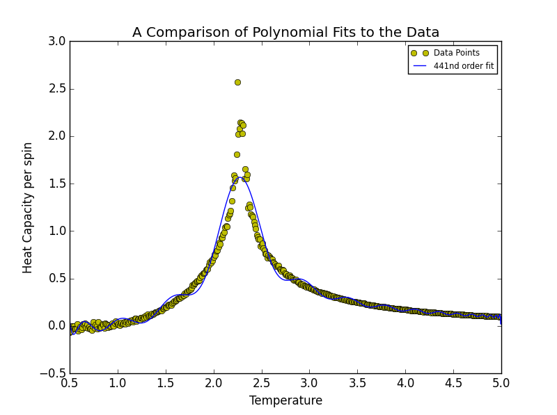
The order of polynomial was increased in powers of 2 until at an order of 512 the polynomial stopped fitting the data. A bisection search was carried out at this stage in order to identify the order of polynomial at which this threshold was reached. This order was determined to be 441. A degree higher than 441 will not fit the data. This behaviour may be seen in the figures below.

Fitting in a Particular Temperature Range

TASK 18: Modify your script from the previous section. You should still plot the whole temperature range, but fit the polynomial only to the peak of the heat capacity! You should find it easier to get a good fit when restricted to this region.


from matplotlib import pylab as pl

import numpy as np

fig = pl.figure()

pl.title("A Comparison of Polynomial Fits to the Data")

HCax = fig.add_subplot(1,1,1)

HCax.set_ylabel("Heat Capacity per spin")

HCax.set_xlabel("Temperature")

degree = 2

data = np.loadtxt("64x64.dat") #assume data is now a 2D array containing two columns, T and C

T = data[:,0] #get the first column

C = data[:,5] # get the fifth column

HCax.plot(T,C, "yo",label = "Data Points") # "yo" parameter determines colour and format of data points

while degree <= 10:

   Tmin = 2.0 #temperature range may be tuned in order to provide best polynomial fit to data

   Tmax = 2.8 #for example

   selection = np.logical_and(T > Tmin, T < Tmax) #choose only those rows where both conditions are true

   peak_T_values = T[selection]

   peak_C_values = C[selection]

   fit = np.polyfit(peak_T_values, peak_C_values, degree) # fit the order polynomial given by variable degree.

   T_range = np.linspace(Tmin, Tmax, 1000) #generate 1000 evenly spaced points between T_min and T_max

   fitted_C_values = np.polyval(fit, T_range) # use the fit object to generate the corresponding values of C

   HCax.plot(T_range, fitted_C_values, label = str(degree) + "nd" + " " + "order" + " " + "fit")

   HCax.legend(loc = 0, fontsize = 'x-small')

   degree += 1

pl.show()

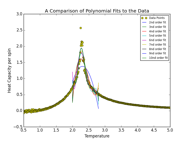
Narrowing the fitting region had the effect such that the order of polynomial required to represent the data decreased significantly. In this instance the degree of polynomial was sequentially by 1 as opposed to being doubled. It was decided that a polynomial of degree 8 marked the best-fit threshold. At first, given that the order was increased to ten, it was thought that both 9th and 10th order polynomials simply misrepresented the data. Such an occurrence was perceived to be similar to the case of the threshold boundary of 441 for the entire range above. However on closer inspection, as may be seen below, it was discovered that the 9th and 10th polynomial fits actually overlap with the 8th order fit.

Finding the Peak in C

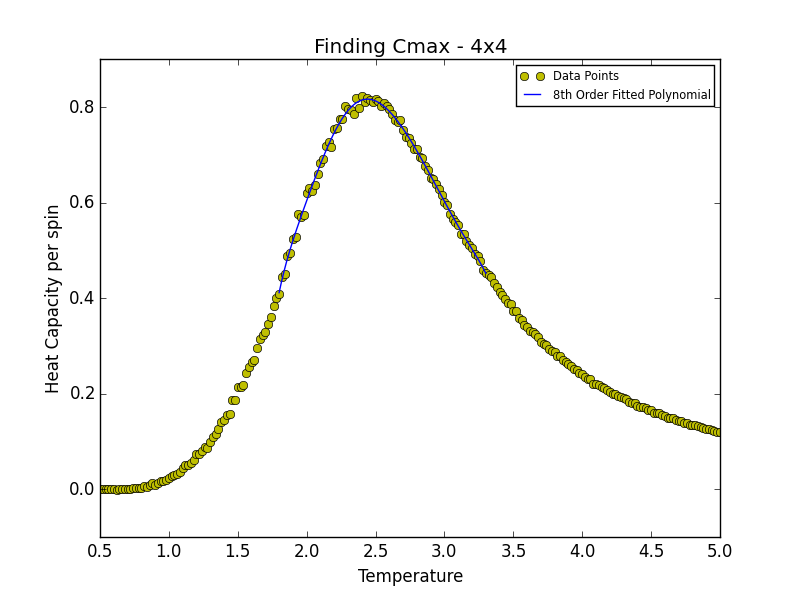
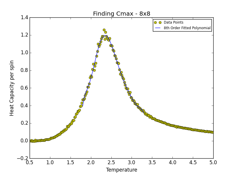
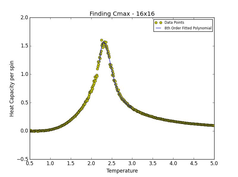
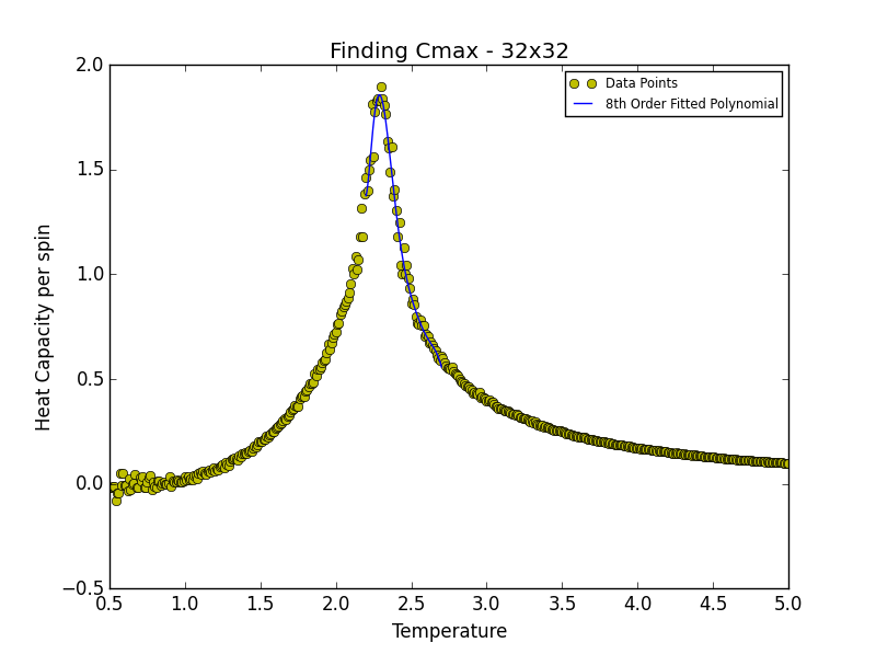
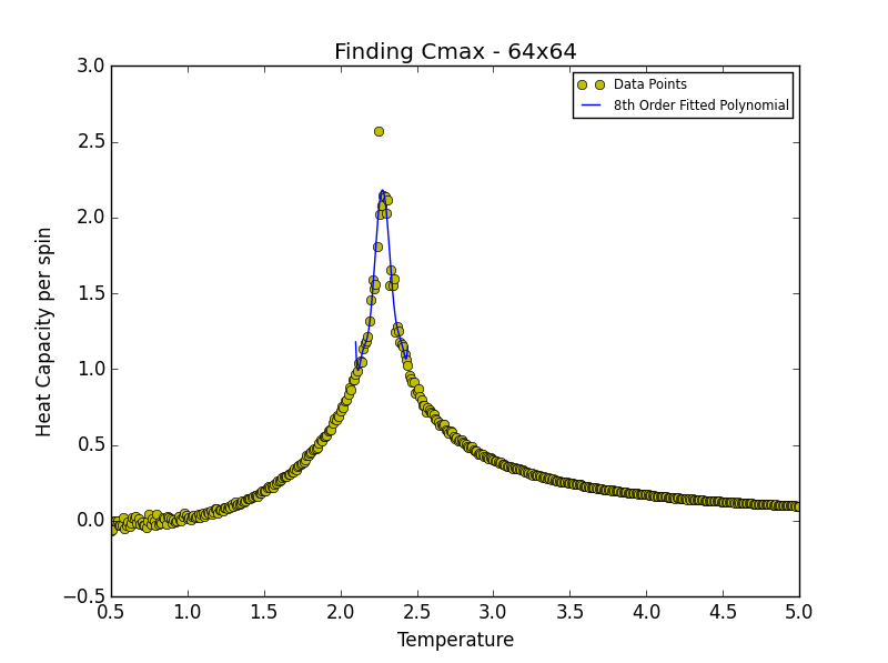
TASK 19: find the temperature at which the maximum in C occurs for each datafile that you were given. Make a text file containing two colums: the lattice side length (2,4,8, etc.), and the temperature at which C is a maximum. This is your estimate of $T_{C}$ for that side length. Make a plot that uses the scaling relation given above to determine $T_{C, \infty}$ . By doing a little research online, you should be able to find the theoretical exact Curie temperature for the infinite 2D Ising lattice. (i) How does your value compare to this? (ii) Are you surprised by how good/bad the agreement is? Attach a PNG of this final graph to your report, and (iii) discuss briefly what you think the major sources of error are in your estimate.

$T_{C, L} = \frac{A}{L} + T_{C, \infty}$ is the scaling relationship that allows one to determine the Curie Temperature of an infinite lattice. By plotting Tmax against the 1/L where L is the lattice size, in the limit that 1/L goes to 0 i.e. when the lattice is infinite, its associated Curie Temperature is obtained as the y-intercept. The polynomial fit for each lattice size is given below. In the case of the 2x2, 4x4 and 8x8 lattices, the temperature range lay between 1.8 and 3.3. For the 16x16 and 32x32 lattices the range was narrowed to 2.2-3.0 while in the case of the 64x64 lattice the range was narrowed further still to 2.2-2.7. This was done in order to obtain a better fit to the data and hence a more accurate estimate of the Curie Temperature for the lattice in question.

Table 7. Curie Temperatures for each Lattice Size.
Lattice Size	Curie Temperature (Reduced Units)
2x2	2.50870871
4x4	2.44114114
8x8	2.34804805
16x16	2.30570571
32x32	2.28488488
64x64	2.27257257


from matplotlib import pylab as pl

import numpy as np

lattice_size = 64

fig = pl.figure()

pl.title("Finding Cmax - " + str(lattice_size) + "x" + str(lattice_size))

HCax = fig.add_subplot(1,1,1)

HCax.set_ylabel("Heat Capacity per spin")

HCax.set_xlabel("Temperature")

degree = 8 #8th degree polynomial chosen as best fit - order at which fit does not improve significantly

Tmin = 2.1 #Range was 1.8 - 3.3 in order to locate Tc for 2x2, 4x4 and 8x8

Tmax = 2.44 #Range narrowed as lattice size increased

data = np.loadtxt("64x64.dat") #assume data is now a 2D array containing two columns, T and C

T = data[:,0] #get the first column

C = data[:,5] # get the fifth column

HCax.plot(T,C, "yo", label = "Data Points")

selection = np.logical_and(T > Tmin, T < Tmax) #choose only those rows where both conditions are true

peak_T_values = T[selection]

peak_C_values = C[selection]

fit = np.polyfit(peak_T_values, peak_C_values, degree) # fit the order polynomial given by variable degree.

T_range = np.linspace(Tmin, Tmax, 1000) #generate 1000 evenly spaced points between T_min and T_max

fitted_C_values = np.polyval(fit, T_range) # use the fit object to generate the corresponding values of C

HCax.plot(T_range, fitted_C_values, label = "8th Order Fitted Polynomial")

HCax.legend(loc = 0, fontsize = 'x-small')

pl.show()

Cmax = np.max(fitted_C_values)

Curie = T_range[fitted_C_values == Cmax] #command print Curie used to obtain Curie Temperature for a given lattice size


from matplotlib import pylab as pl

import numpy as np

Curie_Vals = [2.50870871, 2.44114114, 2.34804805, 2.30570571, 2.28488488, 2.27257257] # List of Curie Temperature values generated from Finding_Curie.py

Recip_Lattice_Lengths = [0.5, 0.25, 0.125, 0.0625, 0.03125, 0.015625] # List of inverse lattice lengths

fit = np.polyfit(Recip_Lattice_Lengths, Curie_Vals, 1)

Recip_Range = np.linspace(0, 0.6, 1000) # value of 0.6 chosen so as to allow the first order fit to extend beyond the final data point

fitted_C_values = np.polyval(fit, Recip_Range)

equation = 'T = ' + str(round(fit[0],4)) + '/L' ' + ' + str(round(fit[1],4))

pl.xlabel('1/L')

pl.ylabel('Curie Temperature')

pl.title('Regression Analysis for Determination of the Curie Temperature')

pl.plot(Recip_Lattice_Lengths, Curie_Vals, "x", label = "Data Points")

pl.plot(Recip_Range, fitted_C_values, label = equation)

pl.legend(loc = 0, fontsize = 'x-small')

pl.show()

(i) and (ii) The theoretical value of the Curie Temperature is known to be 2.269 J ^1,3. The value obtained, 2.2782 J/Kb would seem to be remarkably close given that the value was estimated using data points from lattices comprising less than 4096 spins in total.

(iii) One of the main sources of error for the estimation of the Curie temperature for an infinite lattice is the fact that such small lattices are used for regression. Intuitively one may imagine that a lattice possessing dimensions as small as 2x2 will not be a good representation of an infinite lattice. As such in order to obtain a more precise value it would be better to either exclude these data points (just using four points; 8x8, 16x16, 32x32 and 64x64) or better still perform simulations with larger lattices in their stead. Another approximation used to locate the Curie temperature of the infinite lattice is that the data obtained is best represented by a polynomial function. It could well be the case that the data conforms to a different functional representation.

References

1. L. Onsager, Phys. Rev., 1944, 65, 117-149, DOI:10.1103/PhysRev.65.117 .

2. R. Peierls, Math. Proc. Cambridge, 1936, 32(3), 477-481, DOI:10.1017/S0305004100019174 .

3. H. A. Kramers, G. H. Wannier, Phys. Rev., 60, 252-262, DOI:10.1103/PhysRev.60.252 .

4. Matplotlib, http://matplotlib.org/api/pyplot_api.html [Accessed March 2015].

5. stackoverflow, http://stackoverflow.com/questions/21603585/how-to-add-equation-of-a-line-onto-a-plot-in-python [Accessed March 2015].