Rep:Thermomp4114

Molecular Dynamics Simulations of Simple Liquids Introduction

Molecular dynamic simulations involved studying the motion of a system of particles. Several fundamental elements of a system need to be known in order to achieve this. This includes a knowledge of the interaction potential for the particles and the equations of motion which govern the dynamics of the particles.¹ Once we know the positions, velocities, and forces, of the atoms (which are obtained using statistical) we can calculate various thermodynamic quantities of the system such as temperature and pressure. We must introduce a series of approximations in order for the caluculations to be feasible. Firstly we apply the The Classical Particle Approximation. The schoedinger equation is too complex to solve for a large system of atoms, however if the atoms are treated classically then the positions and and velocities of each can atom can be calculated using Newton's second law (equation 1):

$$\begin{gathered} {\mathbf{F}}_i=m_i{\mathbf{a}}_i=m_i\frac{\mathrm{d}{\mathbf{v}}_i}{\mathrm{d}t}=m_i\frac{{\mathrm{d}}^2{\mathbf{x}}_i}{\mathrm{d}{t}^2} \\ (1) \end{gathered}$$

As there are N atoms and therefore N equations representing each atom a computer is a necessity. The Verlet algorithim is used to solve to Newton's law for all the atoms in the system. In this case time is not continuous but is made discrete, the simulation is thus broeken up into specific timesteps.

The position of atom $i$ at time $t$ is given by ${\mathbf{x}}_i\left(t\right)$.

Positional Verlet algorithim (equation (2)):

$$\begin{gathered} {\mathbf{x}}_i(t+\delta t)\approx 2{\mathbf{x}}_i\left(t\right)-{\mathbf{x}}_i(t-\delta t)+\frac{{\mathbf{F}}_i\left(t\right)}{m_i}\delta t^2 \\ (2) \end{gathered}$$

(Velocity Verlet algorithim (equation (3)):

${\mathbf{v}}_i\left(t\right)$ represents the velocity of that atom at time $t$.

$$\begin{gathered} {\mathbf{v}}_i(t+\delta t)={\mathbf{v}}_i(t+\frac{1}{2}\delta t)+\frac{1}{2}{\mathbf{a}}_i(t+\delta t)\delta t \\ (3) \end{gathered}$$

Put in example of industrial applications

Harmonic Oscillator

The harmonic oscillator illustrates the the accuracy and discrepancies associated with using the velocity Verlet algorithim. Equation (4) is used to model the behavior of the harmonic oscillator in an analytical sense:

$$\begin{gathered} x\left(t\right)=A\cos (\omega t+\varphi ) \\ (4) \end{gathered}$$

$\varphi$ = 0.00
$\omega$ = 1.00
$A$ = 1.00

Graph (1) illustrates the results the analytical solution gave for the relationship between position and time.

Graph 1: Analytical solution of harmonic oscillator

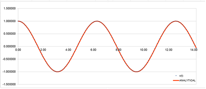
The difference in position between the velocity-verlet solution and analytical solution is represented by an error. Error plotted against time is illustrated by graph (2).

Graph 2: Error vrs Time

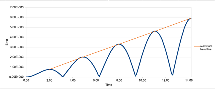
The orange line illustrates the positive trend between error and time. This shows that error is accumulative with time. Each timestep represents a calculation which has an associated error thus as the simulation proceeds the errors will be summed.

The total energy of the system will consist of the sum of kinetic and potential energy. Equation (5) can be used to find kinetic energy of the system:

$$\begin{gathered} E_{\text{k}}=\frac{1}{2}mv(t{)}^2 \\ (5) \end{gathered}$$

When $\mathbf{x}\left(t\right)$ is used in equation (5) the potential energy can be found.

The following graphs represent the difference in change in energy with time when the timestep is varied.

Energy change when a timestep of 0.1 is used	Energy change when a timestep of 0.15 is used	Energy change when a timestep of 0.2 is used

The maximum change in energy for each of the different timesteps is shown in table (1).

Timestep	0.1	0.15	0.2
Max. change in Energy	0.2%	0.6%	1%

The results clearly indicate that a timestep greater than 0.2 will result in an energy change greater than 1%. As the timestep increases as does the maximum error. The timestep defines the number of calculations made in a given time, therefore the shorter the timestep the larger the number of calculations carried out and therefore a more accurate result is produced. The total energy of a real physical system should not change, when modeled numerically there can be fluctuations therefore it is important to monitor this change and ensure that the fluctuations are minimised.

Atomic Forces

The forces an atom experiences is determined by the positions of all the atoms in the system, ${\mathbf{r}}^N$. The Lennard-Jones function accurately sums all the key inter-atomic forces an atoms experiences (U).

$$\begin{gathered} U\left({\mathbf{r}}^N\right)=\sum _i^N\sum _{i\ne j}^N\left\{4ϵ(\frac{{\sigma }^{12}}{r_{ij}^{12}}-\frac{{\sigma }^6}{r_{ij}^6})\right\} \\ (10) \end{gathered}$$

For a single Lennard-Jones interaction:

$\varphi \left(r\right)=4ϵ(\frac{{\sigma }^{12}}{r^{12}}-\frac{{\sigma }^6}{r^6})$

The separation, $r_0$, at which the potential energy is zero is given by:

$0=4ϵ(\frac{{\sigma }^{12}}{r_0^{12}}-\frac{{\sigma }^6}{r_0^6})$

After division by 4 and rearrangement:

$\frac{{\sigma }^6}{r_0^6}=\frac{{\sigma }^6}{r_0^6}$

After further rearrangement and cancelling down:

$r_0=\sigma$

$-\sigma$ is also a solution however this can be disregarded.

In order to calculate the force the following equation is used:

$\mathbf{F}=-\frac{\mathrm{d}\sigma \left(\mathbf{r}\right)}{\mathrm{d}\mathbf{r}}$

After differentiation and simplification:

$\mathbf{F}(r_0)=\frac{24ϵ}{\sigma }$

At equilibrium:

$\frac{\mathrm{d}\varphi \left({\mathbf{r}}_{\mathbf{e}}\right)}{\mathrm{d}\mathbf{r}}$ = 0

$4ϵ(\frac{12{\sigma }^{12}}{r_e^{13}}-\frac{6{\sigma }^6}{r_e^7})$ = 0

After rearrangement:

$r_e=2^{1/6}\sigma$

This value of $r_e$ can now be used to find the well depth:

$4ϵ(\frac{{\sigma }^{12}}{4sigm{a}^{12}}-\frac{{\sigma }^6}{2{\sigma }^6})$

When $\sigma =ϵ=1.0$

$\underset{2\sigma }{\overset{\mathrm{\infty }}{\int }}\varphi \left(r\right)\mathrm{d}r$ = $4ϵ{(\frac{1}{5r^5}-\frac{1}{11r^{1}1})}_2^{\mathrm{\infty }}\simeq -2.48\cdot 10^{-2}$

$\underset{2.5\sigma }{\overset{\mathrm{\infty }}{\int }}\varphi \left(r\right)\mathrm{d}r$ = $\simeq -8.18\cdot 10^{-3}$

$\underset{3\sigma }{\overset{\mathrm{\infty }}{\int }}\varphi \left(r\right)\mathrm{d}r$ = $\simeq -3.29\cdot 10^{-3}$

Periodic Boundary Conditions

• No. of moles in 1 mL of water = 0.056
  
• No. of molecules = moles x Avogadro's constant = 3.37 x 10²²

• 1000 molecules = 1.66 x 10²¹ moles
• Density = mass/vol. = 1
• vol. = mass/density = 2.99 x 10^-20

• Due to periodic boundary condition once the atom leaves the current box it will enter the beginning of an identical box. The atom is at $(0.5,0.5,0.5)$ and thus once it breaches 0.5 in a particular direction it will be at the start of the next box. Using these principles after the atom moves $(0.7,0.6,0.2)$ it will be at the point $(0.2,0.1,0.7)$

Reduced Units

Reduced units are applied to the Lennard-Jones equation to make the calculation more managable.

• distance $r^{*}=\frac{r}{\sigma }$
• energy $E^{*}=\frac{E}{ϵ}$
• temperature $T^{*}=\frac{k_{B}T}{ϵ}$

For argon:

• Distance in real units: r = 1.09 x 10^-7 cm^-1

• Well depth = $ϵ$ = 0.996 KJmol^-1

• T = 180 K

Equilibriation

Simulation Box

As there is a large number of atoms in a discrete volume allowing random assignment of positions could result in atoms overlapping. This would cause an unrealistically high potential as potential is distance dependant (as observed in the Lennard - Jones equation).

• Density is given by the following equation:

$\rho =\frac{n}{v}$

$n$ = 1 (as there is only 1 atom per unit cell)

$v=1.07722^3=1.25$ (lattice spacing = 1.07722)

Thus:

$\rho =\frac{1}{1.25}=0.8$

The length of a side of one fcc unit cell with number density 1.2 would be:

$v=\frac{n}{\rho }$

$n$ = 4 (as there is 4 atoms per unit cell in an fcc lattice)

$v$ = 3.33

$l=v^{-3}=1.49$

• The number of atoms that would be created by the create_atoms command for an fcc lattice would be:

4 x 1000 = 4000

This is due to fact that there is 1 atom per unit cell that yeilds 1000 altogether in simple cubic. Fcc has 4 times the number of atoms per unit cell.

Setting the Properties of Atoms

mass 1 1.0
pair_style lj/cut 3.0
pair_coeff * * 1.0 1.0

The command above has the following purpose:

• The first line sets the mass of all atoms of type '1' to 1.0.
• Line 2 is used to control the Lennard-Jones potential. The value of 3.0 indicates the distance in reduced units upon which the potential is calculated. The potential is distance dependent and falls to 0 at large values of r thus only atoms within a distance of 3.0 are considered. 'lj/cut' defines the cut off point.
• The last line defines the force field constants as 1.0 for all sets of atoms. The * controls the fact that the command is set for all atoms.

The velocity-Verlet is the integration algorithm that can be used when ${\mathbf{x}}_i\left(0\right)$ and ${\mathbf{v}}_i\left(0\right)$ are defined.

### SPECIFY TIMESTEP ###
variable timestep equal 0.001
variable n_steps equal floor(100/${timestep})
variable n_steps equal floor(100/0.001)
timestep ${timestep}
timestep 0.001

### RUN SIMULATION ###
run ${n_steps}
run 100000

The second line (starting "variable timestep...") tells LAMMPS that if it encounters the text ${timestep} on a subsequent line, it should replace it by the value given. In this case, the value ${timestep} is always replaced by 0.001. In light of this, what do you think the purpose of these lines is? Why not just write:

timestep 0.001
run 100000

The codes is in place to ensure that the timestep can be varied but the total time taken for the simulation to run will not change.

Checking equilibration

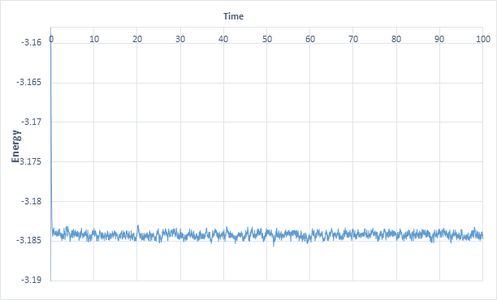
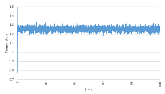
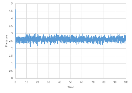
The graphs below illustrate the time it takes for different thermodynamic properties to equilibriate at a timestep of 0.001. The plateau represents the point at which equilibration is achieved.

Energy Vrs Time	Temp vrs Time	Pressure Vrs Time

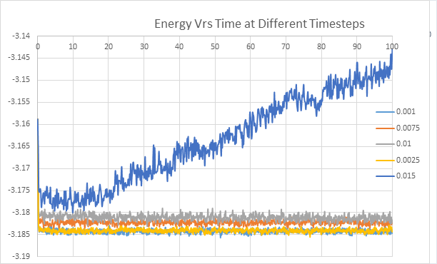
The graph below illustrates the effect changing the timestep has on equilibration. As can be seen from the graph a from below 0.01 a shorter timestep results in a lower energy value for equilibration until 0.0025 where the value of equilibration does not change with lower timestep. This trend is due to the fact that a smaller timestep results in a more accurate result however if it is too small this can over-complicate the calculation (especially when there is a large over-all time). Thus a timestep of 0.0025 is a good balance and therefore ideal. A timestep of 0.025 is too large and results in the system not reaching equilibrium.

Energy Vrs Time with different timesteps

Running Simulations Under Specific Conditions

The following two equations can be used to define the energy of the system:

$E_K=\frac{3}{2}N{k}_{B}T$

$\frac{1}{2}\sum _i{m}_i{v}_i^2=\frac{3}{2}N{k}_{B}T$

The instantaneous tempertaure $T$ will not remain constant throughout the simulation and will fluctuate, it will thus be different to out target temperature $\mathfrak{𝔗}$.

The value of $\gamma$ so that the temperature is correct $T=\mathfrak{𝔗}$ if we multiply every velocity $\gamma$ is as follows:

${\gamma }^2\frac{1}{2}\sum _i{m}_i{v}_i^2=\frac{3}{2}N{k}_B\mathfrak{𝔗}$

${\gamma }^2\frac{3}{2}N{k}_{B}T=\frac{3}{2}N{k}_B\mathfrak{𝔗}$

${\gamma }^{2}T=\mathfrak{𝔗}$

${\gamma }^2=\frac{\mathfrak{𝔗}}{T}$

$\gamma =(\frac{\mathfrak{𝔗}}{T}{)}^{1/2}$

 fix aves all ave/time 100 1000 100000 v_dens v_temp v_press v_dens2 v_temp2 v_press2
run 100000

Within the preceding code:

100 - Nevery: This command results in a sample being taken every 100 steps and being incorporated into the average. 1000 - Nrepreat: Tells the computer how many samples should be used to calculate the average. Nfreq 10 000: At every 10000th timestep an average is calculated.

All thermodynamic properties are calculated by averages that is the necessity for those commands.

Plotting the Equation of State

Density Vrs Temp

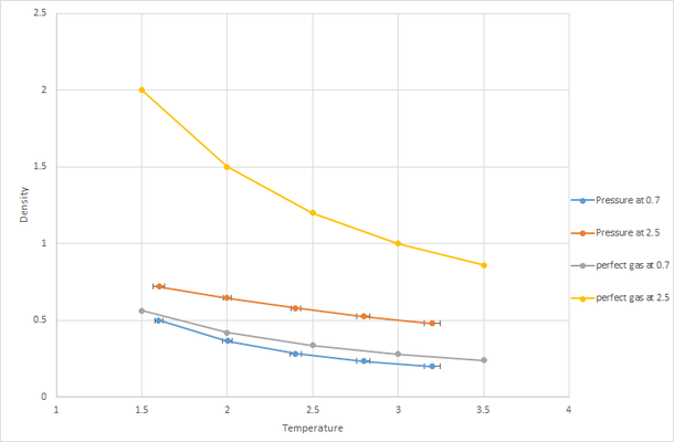
The densities produced from the simulation are lower than for the ideal gas. This is a result of the simulation creating a more realistic picture of how the atoms interact as it takes into account Lennard-Jones potential. In an ideal gas the motion of atoms will be random, chaotic and inter atomic interactions are ignored however in the simulation the atoms will want to minimize their potential and therefore this will drive them to occupy a greater volume thus reducing the density.

Calculating Heat Capacities Using Statistic Physics

Example of input code used:

• Density 0.2
• Temperature 2.0

SPECIFY TIMESTEP

RUN SIMULATION TO MELT CRYSTAL 

run 10000
unfix nve
reset_timestep 0

BRING SYSTEM TO REQUIRED STATE
variable tdamp equal ${timestep}*100
variable ddamp equal ${timestep}*1000
fix nvt all nvt temp ${T} ${T} ${tdamp}
run 10000
reset_timestep 0

MEASURE SYSTEM STATE
unfix nvt
fix nvt all nvt temp ${T} ${T} ${tdamp}
thermo_style custom step etotal temp press density
variable etot equal etotal
variable etot2 equal etotal*etotal
variable temp equal temp
fix aves all ave/time 100 1000 100000 v_etot v_temp v_etot2
run 100000

variable aveetot equal f_aves[1]
variable avetemp equal f_aves[2]
variable aveetot2 equal f_aves[3]
variable varetot equal f_aves[3]-f_aves[1]*f_aves[1]

print "Averages"
print "--------"
print "Temperature: ${avetemp}"
print "Energy Variance: ${varetot}"

The following equation was then used to calculate heat capacity from the results:

$C_V=\frac{\mathrm{V}\mathrm{a}\mathrm{r}\left[E\right]}{k_B{T}^2}$

Heat Capacity Vrs Temp

$C_V=\frac{\partial E}{\partial T}=\frac{\mathrm{V}\mathrm{a}\mathrm{r}\left[E\right]}{k_B{T}^2}=N^2\frac{⟨E^2⟩-{⟨E⟩}^2}{k_B{T}^2}$

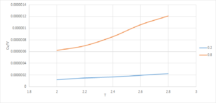
For a fixed number of particles, $N$, a larger density is indicative of a smaller volume. That is why the plot Cv\V Vrs T generally lies at a higher values for a density of 0.8.

From both plots it can been seen that heat capacity increases with temperature. $Var[E]$ increases with temp as at higher temp there are a greater number of accessible rotational, vibration, electronic and kinetic energetic states therefore the system is able to to absorb more energy per rise in temperature.

Structural Properties and the Radial Distribution function

RDF at different phases	Integral of g(r)

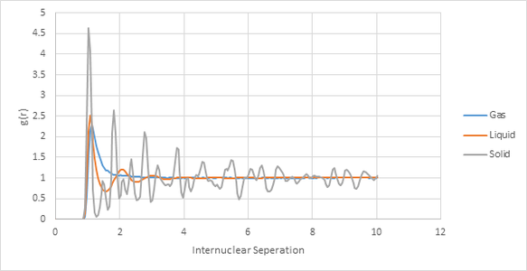
To carry out the RDF calculations temperature was kept constant at 1.2 but density was varied.

Density in reduced units used for each phase:

• Gas = 0.05
• Liquid = 0.8
• Solid = 1.2

The number of peaks for each RDF plot decreases in the order gas<liquid<solid. This reflects the ordering of each phase. A gas has a large degree of disorder and thus produces only peak. The liquid has three peaks which gradually decrease in amplitude, this behavior is due to the fact that the liquid is modeled as central molecule surrounded by shells of other molecules, this initially creates some degree of order. As the simulation continues the molecules become more diffuse so the ordering decreases and thus the amplitude of peaks decrease.

The above plot indicates the positions of the first three peaks. These will correspond to the three closet atoms in the lattice.

• 1.025 will correspond to one of the atoms at the corner of the unit cell neighboring the starting position.
• 1.525 will correspond to one of the atoms in the centre of the face of the cube. (The lattice is fcc)
• 1.825 will correspond to an atom on one of the faces adjacent to the starting point. It cannot be one of the adjacent corners as this would be too large thus it must fall in between the corners and therefore on a face.

Dynamical Properties and the diffusion coefficient

solid	liquid	gas

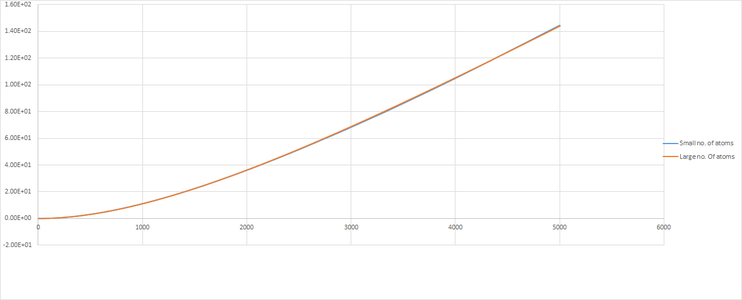
The plot give insight into the displacement of particles as they illustrate mean square displacement with time. There are variations in the shape of the lines for the large number of atoms and small number of atoms, this is due to the variations in positions being averaged for a large number of atoms and thus gives a better indication of the behavior of the system. The difference is very apparent for solid where one can see that the line is much more smooth in the region where the gradient becomes close to 0.

The diffusion constant D was found by calculating the gradient of the line for each phase. The gradient after the line had leveled off was used for the solid.

	D (small System)	D (Large System)
Vapour Phase	0.0304	0.0305
Liquid Phase	0.001	0.0012
Solid Phase	$6x10^{-8}$	$7x10^{-9}$

There is a gradual decrease in D in the order solid<liquid<gas. This fits out chemical intuition; e.g. the motion of a solid would be much more restricted that the motion of a gas.

VACF vrs Temperature

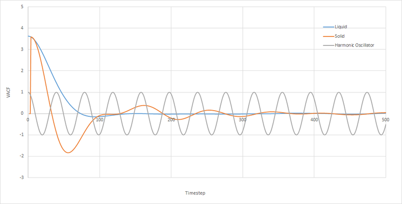
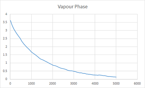
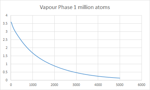
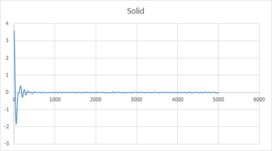
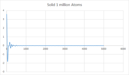
Minima in the VACF plot correspond to points where the atoms collide and change direction. The greater number of minima for a solid is due to the restricted mean square displacement in which the atoms can move, this therefore results in greater collisions as the atoms seek to minimize their potential energy. As a liquid has a greater diffusion coefficient it is able to diffuse away from an atom after a collision, this is why there are fewer minima, the line tends to 0 as the atoms eventually move in opposite directions resulting in velocities cancelling out and therefor the integration becomes 0. The harmonic oscillator is simply a mathematical function without physical meaning therefore it will continue to oscillate around 0 until infinity.

The normalised velocity autocorrelation function for a 1D harmonic oscillator can be evaluated using the equation for a 1D harmonic oscillator.

$C\left(\tau \right)=\frac{\underset{-\mathrm{\infty }}{\overset{\mathrm{\infty }}{\int }}v\left(t\right)v(t+\tau )\mathrm{d}t}{\underset{-\mathrm{\infty }}{\overset{\mathrm{\infty }}{\int }}{v}^2\left(t\right)\mathrm{d}t}$

$x\left(t\right)=A\cos (\omega t+\varphi )$

Differentiation of the displacement function will produce a velocity function:

$\frac{dx}{dt}=-A\omega \sin (\omega t+\varphi )=v(t)$

$v(t+\tau )=-A\omega \sin (\omega t+\omega \tau +\varphi )$

Substitution into velocity autocorrelation:

$C\left(\tau \right)=\frac{\underset{-\mathrm{\infty }}{\overset{\mathrm{\infty }}{\int }}-A\omega \sin (\omega t+\varphi )-A\omega \sin (\omega t+\omega \tau +\varphi )\mathrm{d}t}{\underset{-\mathrm{\infty }}{\overset{\mathrm{\infty }}{\int }}-A\omega \sin (\omega t+\varphi )-A\omega \sin (\omega t+\varphi )\mathrm{d}t}$

Cancelling -A\omega:

$C\left(\tau \right)=\frac{\underset{-\mathrm{\infty }}{\overset{\mathrm{\infty }}{\int }}\sin (\omega t+\varphi )\sin (\omega t+\omega \tau +\varphi )\mathrm{d}t}{\underset{-\mathrm{\infty }}{\overset{\mathrm{\infty }}{\int }}{\sin }^2(\omega t+\varphi )\mathrm{d}t}$

Trigometric relation can simplify equation:

$sin(\omega t+\omega \tau +\varphi )=cos(\omega \tau +\varphi )sin(t\omega )+sin(\omega \tau +\varphi )cos(t\omega )$

$C\left(\tau \right)=\frac{\underset{-\mathrm{\infty }}{\overset{\mathrm{\infty }}{\int }}cos(\omega \tau +\varphi )sin(t\omega )+sin(\omega \tau +\varphi )cos(t\omega )\mathrm{d}t}{\underset{-\mathrm{\infty }}{\overset{\mathrm{\infty }}{\int }}{\sin }^2(\omega t+\varphi )\mathrm{d}t}$

Integration of ansymmetical function results in 0:

$\underset{-\mathrm{\infty }}{\overset{\mathrm{\infty }}{\int }}sin(x)cos(x)\mathrm{d}t=0$

Thus after $cos(t\omega )$is removed from top line the equation simplifies to:

$C\left(\tau \right)=cos(t\omega )$

Vapour Phase	Vapour Phase of 1 million atoms

Solid Phase	Solid Phase of 1 million atoms

Liquid Phase	Liquid Phase of 1 million atoms

	D (small System)	D (Large System)
Vapour Phase	1.64	1.63
Liquid Phase	-0.2215	0.157
Solid Phase	0.254	-0.123

Using the trapezium rule to calculate D from a VACF plot yeilded a similar trend in diffusion coefficients however there was a discrepancy in one of my results. The value of D for a liquid of small number of atoms was smaller and more negative than the solid. This indictaes that using the MSD method is more accurate than VACF. This also indicates that it is more important to use the VACF plot for a large system when calculating D.

References

1. Mark Klarpus, Gregory A. Petsko, (1990) Molecular Reaction Dynamics in Biology, 347, 631-9, doi:10.1038/347631a0