Introduction to the Ising Model

The Ising model is a physical model describing ferromagnetic behaviour, where the spins in a material align in a particular direction. The most likely configuration is given when the free energy of the lattice is minimised. This is done through internal energy minimisation and entropy maximisation as $A = U - T S$ . Parallel alignment of spins, minimises internal energy but also minimises entropy, thus a compromise must be struck.

In the model, the spins can either be up (+1) or down (-1). In the 2D Ising Model that was constructed, the spins were orientated in a grid with their spin pointing either up or down. The constraints of the model were as follows:

1. Only the spins adjacent to a particular spin would contribute to the overall energetic contribution, when no external magnetic field is applied.

2. The overall interaction energy is given as $- \frac{1}{2} J \sum_{i}^{N} \sum_{j \in n e i g h b o u r s (i)} s_{i} s_{j}$ , where $J$ is a constant controlling strength of interaction. $j \in n e i g h b o u r s (i)$ shows that spin $j$ lies in a lattice cell adjacent to spin $i$ . The sum is divided by 2 to avoid double counting the number of interactions.

3. Periodic boundary conditions are applied, so that the system can be treated as an infinite 2D lattice.

Task 1: Show that the lowest possible energy for the Ising model is -DNJ, where D is the number of dimensions and N is the total number of spins. What is the multiplicity of this state? Calculate its entropy.

The lowest possible energy is obtained when all the spins are parallel, therefore $s_{i} = s_{j}$ so $s_{i} \times s_{j} = + 1$ and therefore in 1D $E = - \frac{1}{2} J \times N \times 2$ as the interactions are doubly counted. This gives -1NJ as the energy.

In 2D, there are 2 times more neighbours than in 1D so $E = - \frac{1}{2} J \times 2 N \times 2$ and therefore $E = - 2 N J$ . In 3D, there are 3 times more neighbours than in 1D so $E = - \frac{1}{2} J \times 3 N \times 2$ and therefore $E = - 3 N J$ .

In D dimensions, there are D times more neighbours than in 1D so $E = - D N J$ .

The multiplicity of this state is two are there are two states with the minimum energy - one where all the spins are parallel and up and the other when all the spins are parallel and down. Therefore the entropy of this state is equal to $k_{B} \times l n (2)$ which is $9.57 \times 1 0^{- 24} J K^{- 1}$

Task 2: Imagine that the system is in the lowest energy configuration. To move to a different state, one of the spins must spontaneously change direction ("flip"). What is the change in energy if this happens (D=3,\ N=1000)? How much entropy does the system gain by doing so?

The energy of the lowest energy state is equal to -3000J. By removing one spin, 6 interactions are lost and by flipping the spin and putting it back in, another 6 interactions are lost. Therefore the energy of the flipped spin state is equal to -2988J. The entropy of this new flipped spin system is equal to $k_{B} \times l n (2000)$ as the multiplicity of the flipped state is 2000. This is because there are 1000 different spins that one could flip in the lattice to give this energy and there are another 1000 possibilities when all the spins are flipped the other way to give the same energy and are indistinguishable until an external magnetic field is applied.

Task 3: Calculate the magnetisation of the 1D and 2D lattices in figure 1. What magnetisation would you expect to observe for an Ising lattice with D = 3,\ N=1000 at absolute zero?

In the 1D lattice, M = +1. In the 2D lattice, M = +1. For a 3D lattice with 1000 spins in the lowest energy state, M = +1000 or -1000 as all the spins can either be spin up or spin down.

Calculating the energy and magnetisation

Task 1: Complete the functions energy() and magnetisation(), which should return the energy of the lattice and the total magnetisation, respectively. In the energy() function you may assume that J=1.0 at all times (in fact, we are working in reduced units in which $J = k_{B}$ , but there will be more information about this in later sections). Do not worry about the efficiency of the code at the moment — we will address the speed in a later part of the experiment.

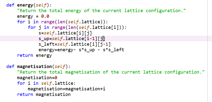
The energy and magnetisation functions were written as shown below. The energy function seemed to be correct and was created through summing through all the interactions of each spin with the spin directly to the left and above, allowing the [-1] index notation to be used in the case where the lattice being considered had a zero index. This method ensured that all the interactions in the lattice were summed and the factor of 0.5 could be removed as I was no longer double counting the interactions. The first for loop, looped through all the indices of the rows and the second looped through the indices for the columns, before calculating the interactions between adjacent spins to the left and above. The magnetisation function was incorrect as each element of self.lattice produced each row of the lattice instead of each individual spin in the lattice. Therefore another for loop was required to loop through the spins of each row and summing their values by converting them to floating point numbers. I did not screenshot the adapted correct magnetisation method unfortunately.

Task 2: Run the ILcheck.py script from the IPython Qt console using the command

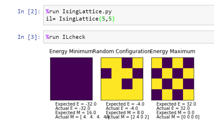
The results of the check test are shown below. The actual magnetisations when repeated with the correct magnetisation function were 16.0 for the minimum energy configuration, 8.0 for the random energy configuration and 0.0 for the maximum energy configuration.

Introduction to Monte Carlo Simulation

Task 1: How many configurations are available to a system with 100 spins? To evaluate these expressions, we have to calculate the energy and magnetisation for each of these configurations, then perform the sum. Let's be very, very, generous, and say that we can analyse $1 \times 1 0^{9}$ configurations per second with our computer. How long will it take to evaluate a single value of ${⟨ M ⟩}_{T}$ ?

The number of configurations available to a system with 100 spins is $2^{100}$ as there are two possible spins available for each spin in the lattice. At a rate of $1 \times 1 0^{9} s^{- 1}$ , the time needed for a computer to process this number of configurations is $\frac{2^{100}}{1 0^{9}}$ , which gives an answer of $1.27 \times 1 0^{21} s$ , which is definitely far too long.

Task 2: Implement a single cycle of the above algorithm in the montecarlocycle(T) function. This function should return the energy of your lattice and the magnetisation at the end of the cycle. You may assume that the energy returned by your energy() function is in units of k_B! Complete the statistics() function. This should return the following quantities whenever it is called: $< E >$ , $< E^{2} >$ , $< M >$ , $< M^{2} >$ , and the number of Monte Carlo steps that have elapsed.

The Monte Carlo Step method was created using the following steps. The variable energy0 took the initial energy of the system. The following 2 lines assigned random coordinates, which was then used in the line after to flip the spin of that lattice point. the variable energy1 took the final energy of the system after one spin had been flipped. DeltaE took the difference in energy between the two states. The if statement afterwards said that if the change in energy was positive and the random number was larger than the Boltzmann factor of the system, then revert the system back to the original state and add it to the variables summing energy, square of energy, magnetisation and square of magnetisation. Otherwise, if the previously mentioned conditions were not satisfied, then add it to the variables summing energy, square of energy, magnetisation and square of magnetisation.

The use of random numbers and probabilities to sample through a system instead of systematically going through every possible configuration is the Monte Carlo method. Since, if the change in energy was high in magnitude and positive, then the Boltzmann factor is likely to be close to zero. The probability of the random number being larger than the Boltzmann factor is very high. In this case, the final state will be reverted back to the initial state and the initial state values will be added to the variables summing energy, magnetisation and their squares. At the other extreme, if the change in energy is very small in magnitude and positive, the Boltzmann factor will be close to 1. The probability of the random number being larger than the Boltzmann factor will be very low and so the final state will be added to the variables summing energy, magnetisation and their squares. The method returns the energy and magnetisation at each step.

The statistics method takes the sums of the energy, magnetisation and their squares and divides them all by the number of Monte Carlo cycles which have occurred to give average values.

The Monte Carlo Step and statistics methods are shown below and worked correctly:

Task 3: If $T < T_{C}$ , do you expect a spontaneous magnetisation (i.e. do you expect $⟨ M ⟩ \neq 0$ )? When the state of the simulation appears to stop changing (when you have reached an equilibrium state), use the controls to export the output to PNG and attach this to your report. You should also include the output from your statistics() function.

Yes I would expect spontaneous magnetisation as at very low temperatures below the Curie Temperature, the system is dominated by energetics and not entropy. As the energetically most stable state is when all the spins are parallel, this would result in overall magnetisation. The exported graph is shown below. The results from the statistics method were unable to be exported as they all showed as zero due to a Windows error, which was unable to be fixed at the time.

Accelerating the code

Task 1: Use the script ILtimetrial.py to record how long your current version of IsingLattice.py takes to perform 2000 Monte Carlo steps. This will vary, depending on what else the computer happens to be doing, so perform repeats and report the error in your average!

This shows that the mean time taken to complete 2000 cycles is quite large and the spread of the times is also fairly large.

Task 2: Look at the documentation for the NumPy sum function. You should be able to modify your magnetisation() function so that it uses this to evaluate M. The energy is a little trickier. Familiarise yourself with the NumPy roll and multiply functions, and use these to replace your energy double loop (you will need to call roll and multiply twice!).

The magnetisation method and most of the energy method can be seen below.

def energy(self):
    "Return the total energy of the current lattice configuration."
    energy = -np.sum(np.multiply(self.lattice, np.roll(self.lattice, (1,0)))) - np.sum(np.multiply(self.lattice, np.roll(self.lattice, (1,1))))
    return energy

def magnetisation(self):
    "Return the total magnetisation of the current lattice configuration."
    magnetisation = np.sum(self.lattice)
    return magnetisation

Task 2: Use the script ILtimetrial.py to record how long your new version of IsingLattice.py takes to perform 2000 Monte Carlo steps. This will vary, depending on what else the computer happens to be doing, so perform repeats and report the error in your average!

This shows that the new mean time taken to run 2000 cycles has been sped up by about a factor of at least 10 and the spread of these times is also smaller, so the reliability of the code to run at that speed is also high.

The Effect of Temperature

Task 1: The script ILfinalframe.py runs for a given number of cycles at a given temperature, then plots a depiction of the final lattice state as well as graphs of the energy and magnetisation as a function of cycle number. This is much quicker than animating every frame! Experiment with different temperature and lattice sizes. How many cycles are typically needed for the system to go from its random starting position to the equilibrium state? Modify your statistics() and montecarlostep() functions so that the first N cycles of the simulation are ignored when calculating the averages. You should state in your report what period you chose to ignore, and include graphs from ILfinalframe.py to illustrate your motivation in choosing this figure.

The adapted code for the Monte Carlo step method is shown below. The process for giving the equilibrium energies was to create a comparison between three different samples in the most recent cycles in the past, each of the same size proportional to the size of the lattice. If the standard deviation of these three samples was smaller than 0.01 multiplied by the Temperature, then the system was deemed to be in a state of equilibrium and the energies were allowed to be summed up. Having also observed across many simulations that after 80000 cycles, most systems were in equilibrium, an or statement was included so that if the number of cycles exceeded 80000, then the system was also deemed to be in equilibrium and all energies beyond this point were summed up. The variable newn was created to count the number of states which were deemed to be in the equilibrium state.

def montecarlostep(self, T):
    self.n_cycles = self.n_cycles + 1
    # complete this function so that it performs a single Monte Carlo step
    energy0 = self.energy()
    #the following two lines will select the coordinates of the random spin for you
    random_i = np.random.choice(range(0, self.n_rows))
    random_j = np.random.choice(range(0, self.n_cols))
    self.lattice[random_i][random_j] = -self.lattice[random_i][random_j]
    energy1 = self.energy()
    deltaE = energy1-energy0
    #the following line will choose a random number in the range [0,1) for you
    random_number = np.random.random()

    self.list = self.list + [self.energy()]
    weight = 8
    threshold = weight * self.n_rows * self.n_cols
    if self.n_cycles > threshold and self.avgE == False:
        s1 = np.mean(np.array(self.list[(self.n_cycles - 3*threshold):int(self.n_cycles - 2*threshold)]))
        s2 = np.mean(np.array(self.list[int(self.n_cycles - 2*threshold):int(self.n_cycles - threshold)]))
        s3 = np.mean(np.array(self.list[int(self.n_cycles - threshold):self.n_cycles]))
        if np.std(np.array([s1,s2,s3])) < 0.01*T:
            self.avgE = True
               
    if deltaE>0 and random_number > np.exp(-deltaE/T):
        self.lattice[random_i][random_j] = - self.lattice[random_i][random_j]
        if self.avgE == False:
            self.list.append(energy0)
        magnetisation=self.magnetisation()
        if self.avgE == True or self.n_cycles > 80000:
            self.newn+=1
            self.E = self.E + float(energy0)
            self.E2 = self.E2 + float(energy0**2)
            self.M = self.M + float(magnetisation)
            self.M2 = self.M2 + float(magnetisation**2)
        return float(energy0), float(magnetisation)
                   
    else:
        self.list.append(energy1)
        magnetisation=self.magnetisation()
        if self.avgE == True or self.n_cycles > 80000:
            self.newn+=1
            self.E = self.E + float(energy1)
            self.E2 = self.E2 + float(energy1**2)
            self.M = self.M + float(magnetisation)
            self.M2 = self.M2 + float(magnetisation**2)
        return float(energy1), float(magnetisation)

def statistics(self):
    # complete this function so that it calculates the correct values for the averages of E, E*E (E2), M, M*M (M2), and returns them
    print(self.n_cycles-self.newn)
    return (self.E/self.newn, self.E2/self.newn, self.M/self.newn, self.M2/self.newn)

Task 2: Use ILtemperaturerange.py to plot the average energy and magnetisation for each temperature, with error bars, for an 8x8 lattice. Use your intuition and results from the script ILfinalframe.py to estimate how many cycles each simulation should be. The temperature range 0.25 to 5.0 is sufficient. Use as many temperature points as you feel necessary to illustrate the trend, but do not use a temperature spacing larger than 0.5. The NumPy function savetxt() stores your array of output data on disk — you will need it later. Save the file as 8x8.dat so that you know which lattice size it came from.

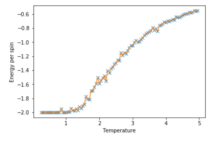
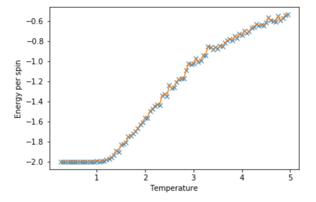
The average energy and magnetisation per spin graphs for each temperature were plotted below for an 8x8 lattice. The standard error was calculated for each temperature using the following formulae:

$V a r [X] = ⟨ X^{2} ⟩ - {⟨ X ⟩}^{2}$

$s_{X} = \sqrt{V a r [X]}$

$σ_{X} = \frac{s_{X}}{\sqrt{n}}$

where $V a r [X]$ is the Variance of a given variable X, $s_{X}$ is the standard deviation of a given variable X and $σ_{X}$ is the standard error for a given variable X.

The error bars were plotted using standard error but were too small to be observed. As most systems reach equilibrium by 80000 cycles, a runtime of 100000 cycles was chosen for each temperature.

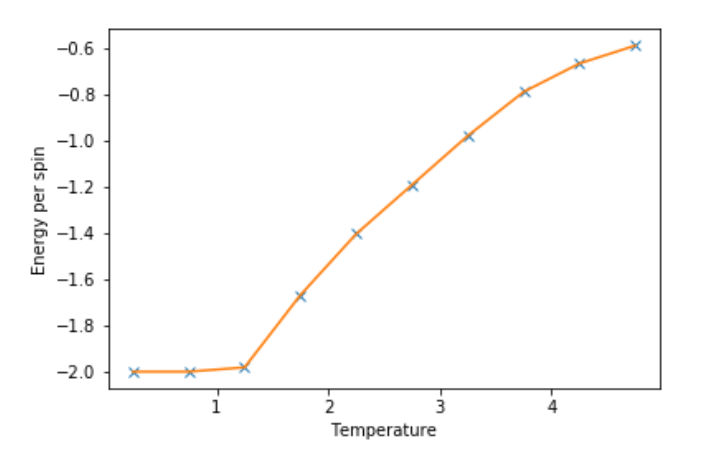
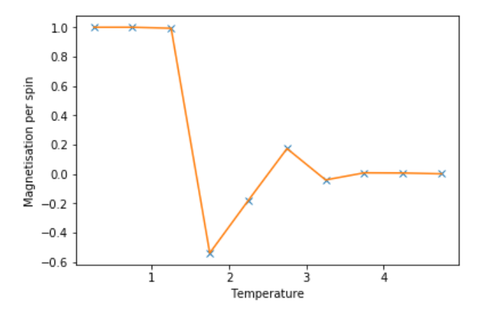
A temperature spacing of 0.5 was used but the graph did not illustrate the trend as best as possible. Therefore a smaller temperature spacing of 0.05 was chosen the graphs for this can be seen below:

The first graph of Energy per spin against Temperature, shows a deviation from the energetically most stable state with increasing Temperature due to the increasing effect of Entropy giving the equilibrium state with the most negative free energy. The second graph shows the deviation from being spontaneously magnetic to having no net magnetic moment beyond the Curie Temperature.

The smaller lattice sizes such as 2x2 and 4x4 have lower energy barriers to go from all spins up to all spins down at low temperatures as the random thermal fluctuations have a greater effect on the energy of the system. Therefore, the systems in smaller lattice sizes are seen to oscillate more between +1 and -1 Magnetisations per spin before going to zero at the Curie Temperature. Larger lattice sizes such as 16x16 and 32x32 have higher energy barriers which are less easily overcome due to the weaker effect of random thermal fluctuations on the overall energy of the system. Therefore, systems in larger lattice sizes are seen to remain at around +1 Magnetisation per spin before reaching zero beyond the Curie Temperature.

The Effect of System Size

Task 1: Repeat the final task of the previous section for the following lattice sizes: 2x2, 4x4, 8x8, 16x16, 32x32. Make sure that you name each datafile that your produce after the corresponding lattice size! Write a Python script to make a plot showing the energy per spin versus temperature for each of your lattice sizes. Hint: the NumPy loadtxt function is the reverse of the savetxt function, and can be used to read your previously saved files into the script. Repeat this for the magnetisation. As before, use the plot controls to save your a PNG image of your plot and attach this to the report. How big a lattice do you think is big enough to capture the long range fluctuations?

Below are the Energy and Magnetisation per spin graphs against Temperature for 32x32 lattice size. The other lattice sizes can be found in Temperature_Dependence.ipynb. It was found that smaller lattice sizes could be more easily perturbed out of local minima and towards the global minimum. It was also found that larger lattice sizes were more likely to be trapped in local minima as the wells are deeper for a larger lattice and the random fluctuations would not have enough strength to push you out of local minima and towards the global minimum. I think that a lattice size of 16x16 would be big enough to capture the long range fluctuations. Beyond this, the fluctuations become less easily observed, as the size of the fluctuations is proportional to $\frac{1}{\sqrt{N}}$ ^[1].

Determining the Heat Capacity

Task 1: By definition,

C = $\frac{\partial ⟨ E ⟩}{\partial T}$

From this, show that

C = $\frac{V a r [E]}{k_{B} T^{2}}$

(Where $V a r [E]$ is the variance in E.)

The average energy $< E >$ is equal to the internal energy $U$ in this scenario as the system is fully isolated and the definition of heat capacity is $C = \frac{\partial U}{\partial T}$ .

The variance in internal energy, Var(U) is given as: $V a r (U) = - \frac{\partial U}{\partial β}$ , where $β = \frac{1}{k T}$ , as the variance of internal energy is defined as the rate of change of internal energy with respect to thermal fluctuations. The reason for the negative sign is because as Temperature increases, we expect the number of thermal fluctuations and therefore Variance to increase as well. As β has an inverse relationship with Temperature, therefore we need to include a negative sign.

$C = \frac{\partial U}{\partial T} = \frac{\partial U}{\partial β} \frac{\partial β}{\partial T} = \frac{- V a r (U)}{- k_{B} T^{2}} = \frac{V a r (U)}{k_{B} T^{2}}$

Task 2: Write a Python script to make a plot showing the heat capacity versus temperature for each of your lattice sizes from the previous section. You may need to do some research to recall the connection between the variance of a variable, $V a r [X]$ , the mean of its square $⟨ X^{2} ⟩$ , and its squared mean ${⟨ X ⟩}^{2}$ . You may find that the data around the peak is very noisy — this is normal, and is a result of being in the critical region. As before, use the plot controls to save your a PNG image of your plot and attach this to the report.

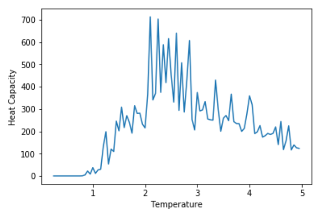
The Variance was calculated using the formula previously mentioned and the graph of Heat Capacity against Temperature for a 32x32 lattice size is shown below. The other graphs of Heat Capacity against Temperature for other lattice sizes can be found in Heat_Capacities.ipynb

This shows that the Heat Capacity increases with Temperature up to the Curie Temperature, after which the Heat Capacity decreases at a slower rate afterwards. Around the Curie Temperature, the Heat Capacity is very noisy due to large thermal fluctuations.

Locating the Curie Temperature

Task 1: A C++ program has been used to run some much longer simulations than would be possible on the college computers in Python. You can view its source code here if you are interested. Each file contains six columns: $T, E, E^{2}, M, M^{2}, C$ (the final five quantities are per spin), and you can read them with the NumPy loadtxt function as before. For each lattice size, plot the C++ data against your data. For one lattice size, save a PNG of this comparison and add it to your report — add a legend to the graph to label which is which. To do this, you will need to pass the label="..." keyword to the plot function, then call the legend() function of the axis object

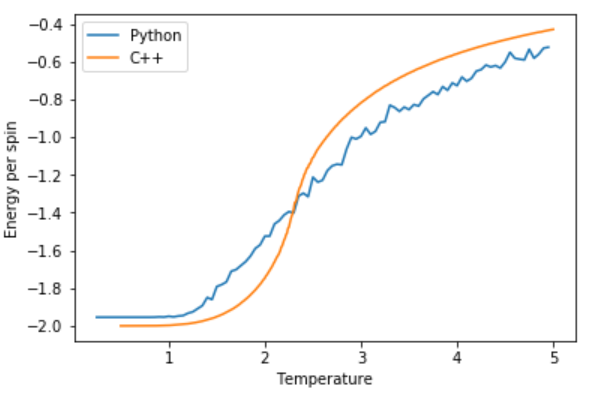
The comparison between the C++ and Python processed data for the Heat Capacity against Temperature is shown below for a 32x32 lattice size. Other lattice size comparisons can be seen in C++_comparison.ipynb and the trend found is that for the smaller lattice sizes, the C++ and Python data match more closely.

The C++ data has a a smoother Energy per spin profile compared to the Python data but both become positive and more unstable energetically around the Curie Temperature.

For the C++ data, the system remains magnetised for longer in a large lattice size, until it reaches the Curie Temperature and the magnetisation fluctuates around zero. For the Python data, the system fluctuates more at lower temperatures until it reaches the Curie Temperature and fluctuates heavily around zero.

For the C++ data, the Heat Capacity has a strong peak at the Curie Temperature but with the Python data, the Heat Capacity peaks around the Curie Temperature but not as strongly as the C++ data and is much noisier.

For all of the comparisons, smaller lattice sizes using the Python data, matched with the C++ data much better than at higher lattice sizes like 32x32 above.

Task 2: Write a script to read the data from a particular file, and plot C vs T, as well as a fitted polynomial. Try changing the degree of the polynomial to improve the fit — in general, it might be difficult to get a good fit! Attach a PNG of an example fit to your report.

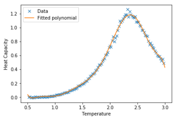
A script was written to read data from the 2x2 lattice size C++ file and plot C vs T and a fitted ninth order polynomial, which is shown below:

For smaller lattice sizes like 2x2, lower order polynomials could be used to match the Heat Capacities. In general, higher order polynomials would be needed to match the Heat Capacities drawn from Python, due to the more irregular nature of the function and its noise.

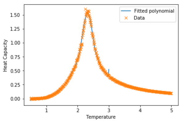
Task 3: Modify your script from the previous section. You should still plot the whole temperature range, but fit the polynomial only to the peak of the heat capacity! You should find it easier to get a good fit when restricted to this region.

Below is the code written to read data from the 16x16 lattice size C++ file and plot, C vs T and a fitted polynomial of order 20. The graph is also shown. The scripts for the other lattice sizes can be found in C++_comparison.ipynb

data16 = np.loadtxt("16x16C.dat") #16x16 C++ generated file
T16 = data16[:,0] #get the first column
C16 = data16[:,5] # get the fifth column

Tmin16 = 0.5 
Tmax16 = 3.0 #range from 0.5 to 3.0

selection16 = np.logical_and(T16 > Tmin16, T16 < Tmax16) #choose only those rows where both conditions are true
peak_T_values16 = T16[selection16]
peak_C_values16 = C16[selection16]

fit16 = np.polyfit(peak_T_values16, peak_C_values16, 20) #twentieth order polynomial
T_range16 = np.linspace(Tmin16, Tmax16, 1000) #generate 1000 evenly spaced points between T_min and T_max
fitted_C_values16 = np.polyval(fit16, T_range16)

plt.plot(T_range16,fitted_C_values16, label='Fitted polynomial')
plt.plot(T16,C16,marker='x', linestyle=, label='Data')
xlabel('Temperature')
ylabel('Heat Capacity')
plt.legend()

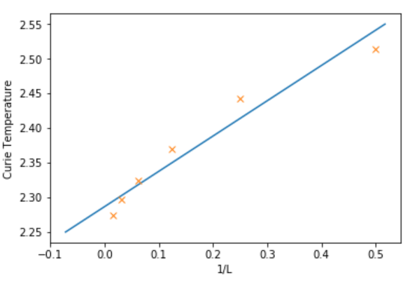
Task 4: Find the temperature at which the maximum in C occurs for each datafile that you were given. Make a text file containing two columns: the lattice side length (2,4,8, etc.), and the temperature at which C is a maximum. This is your estimate of T_C for that side length. Make a plot that uses the scaling relation given above to determine $T_{C, \infty}$ . By doing a little research online, you should be able to find the theoretical exact Curie temperature for the infinite 2D Ising lattice. How does your value compare to this? Are you surprised by how good/bad the agreement is? Attach a PNG of this final graph to your report, and discuss briefly what you think the major sources of error are in your estimate.

The data file with the lattice side length and Curie Temperatures is called Curie_Temperatures.dat. There was found to be an inversely linear relationship between lattice side length and Curie Temperature and so $T_{C}$ was plotted against $\frac{1}{L}$ with the y intercept being equal to $T_{C, \infty}$ . Therefore $T_{C, \infty}$ was found to be 2.291 (3 dp). This was compared to the theoretical value for the Curie Temperature of a 2D Ising Lattice of 2.269 (3 dp) ^[2] and there was a 0.97% difference between the values. The major sources of error in my estimate are likely to be due to a less than 100% efficient method of detecting the equilibrium state at each temperature, combined with greater than normal thermal fluctuations once in the equilibrium state.

Conclusion

In this lab, a 2D Ising model for ferromagnetism was created. Creating energy and magnetisation methods, the energy and magnetisation of the system was able to be measured. Using the Monte Carlo Method, starting from a random configuration, the configuration with lowest energy was found. The simulation was repeated across many temperatures, to show the temperature dependence of the system. It was found that the lattice at low temperatures was dominated by energetics and so the lowest possible energy configuration where all the spins were parallel was the equilibrium state. This state also had the lowest entropy. However, as temperature was increased, a balance had to be struck to maximise entropy, in order to minimise the free energy of the system. Thus the energy of the system was found to increase with Temperature. Beyond the Curie Temperature, there was no spontaneous magnetisation, meaning that the magnetisation per spin for $T < T_{C}$ was either +1 or -1 and beyond the Curie Temperature, the magnetisation per spin was zero. The size of the lattice was varied and it was found that the energy barriers and transition states were higher for larger lattices. Furthermore, larger lattice sizes had deeper potential wells, meaning it would be difficult to get out of local minima to reach the global minimum. The equation for heat capacity was derived showing its dependence on the variance of the energy and was found to have a maximum at the Curie Temperature. The C++ data provided was found to be much less noisy than the data created using Python as there were many more cycles taken for each temperature. High order polynomials were fitted to the heat capacity graphs to estimate the maximum point, which corresponded to the Curie Temperature. Using the data of the Curie Temperatures of different lattice sizes, it was found that there was a linear relationship between Curie Temperature and 1/L, where L is the lattice side length. From this graph, the y-intercept was $T_{C, \infty}$ and so it was calculated to be 2.291, which had a 0.97% difference from the literature value of 2.269.

↑ Statistical Physics, Section 3: Fluctuations and Response, https://www2.ph.ed.ac.uk/~mevans/sp/sp3.pdf
↑ https://en.wikipedia.org/wiki/Square-lattice_Ising_model

[1] Statistical Physics, Section 3: Fluctuations and Response, https://www2.ph.ed.ac.uk/~mevans/sp/sp3.pdf

[2] ttps://en.wikipedia.org/wiki/Square-lattice_Ising_model

[1]

[2]