Rep:Sn3215 liquid sim final

Abstract

Several Lennard-Jones gases, liquids, solids, and fluids have been analyzed using the LAAMPS molecular dynamics package, and the calculations of thermodynamic and structural properties including the equation of state, heat capacity, radial distribution function, mean-squared displacement, and velocity autocorrelation function, have been demonstrated. As an additional experiment, three systems of liquid interfaces were simulated with variations in particle mass, lattice densities, and simulation boundary conditions.

Introduction

Molecular simulation is an invaluable tool in modern scientific research. Simulations allow researchers to not only calculate properties and structures of molecular systems, but can allow users to visualize the structure and dynamics of systems that are too small to resolve otherwise. Molecular simulations have enabled the compilation of large amounts of data, for example in the properties of semiconductors and quantum dots, and in characterizing mechanisms for chemical reactions ^[1].

Molecular dynamics simulations study atoms and molecules in defined potential fields, which can take molecular interactions, electrostatics, and even quantum effects into account. One of the most popular potential fields to use is the Lennard-Jones potential, which includes Pauli electron-election repulsion, and Van der Waals attraction. The simple form of the Lennard-Jones field reduces computational time, and the potential field has been found to produce accurate results for small-scale simulations of inert particles in the solid, liquid, and gas phases.

Many systemic properties can be derived from particles in a Lennard-Jones field. Aside from standard thermodynamic variables, one can extract information such as equations of state, heat capacities, radial distribution functions, and diffusion coefficients from simulations of Lennard-Jones systems. Additionally, the dynamic motion of the system can be rendered using visualization software, allowing visual analysis of the time-evolution of the system.

There are several molecular dynamics software packages available for public use. Among them, LAMMPS is a flexible package that is able to simulate solids, liquids, and gases in atomic, polymeric, biological, metallic, coarse-grained and granular systems under a variety of force-fields and boundary conditions ^[2].

In this experiment, we investigate several properties of Lennard-Jones systems from a molecular dynamics perspective. We will use the LAMMPS molecular dynamics package for all simulations, and visualize selected trajectories in VMD.

Aims and Objectives

This wiki aims to investigate some of the fluid dynamics capabilities of the LAMMPS simulation package. It will specifically focus on the initialization and analysis of simple Lennard-Jones fluids and solids, and will illustrate LAMMPS input script syntax, parameter determination, and data extraction.

The wiki will progress through a series of example experiments, each of which will emphasize a different aspect of LAMMPS and its applications.

1. Simple fluid simulations with different timesteps - investigating equilibration.

2. Plotting equations of state - setting conditions, and extracting thermodynamic data.

3. Calculating the heat capacity - data extraction and analysis.

4. Finding the radial distribution function - trajectory outputs.

5. Calculating the diffusion coefficient via the mean-squared displacement and the velocity autocorrelation function - dynamical properties.

6. Extension - dynamics of multi-component systems.

Theory

The Velocity Verlet Algorithm

The Velocity Verlet algorithm is a commonly used algorithm for simulating molecular motion in simulations. Its defining feature is its ability to calculate both the velocity and the acceleration of a particle in the same instance, which enables the observation of quantities such as the kinetic energy of the system.

The Velocity Verlet algorithm is implemented as below:

Calculate the velocity half a step in the future using a Taylor expansion: $\vec{v} (t + \frac{1}{2} Δ t) = \vec{v} (t) + \frac{1}{2} \vec{a} (t) Δ t .$
Calculate the position one step in the future using the half-step velocity: $\vec{x} (t + Δ t) = \vec{x} (t) + \vec{v} (t + \frac{1}{2} Δ t) Δ t .$
Calculate the full-step acceleration $\vec{a} (t + Δ t)$ from the interaction potential using $\vec{x} (t + Δ t) .$
Calculate the full-step velocity: $\vec{v} (t + Δ t) = \vec{v} (t + \frac{1}{2} Δ t) + \frac{1}{2} \vec{a} (t + Δ t) Δ t .$ ]]

Since the Taylor series expansion is limited to two terms, the error in each calculation is limited:

$E r r o r \leq δ t^{3} .$

where $δ t$ is the timestep.

The Timestep

As the margin of error for each calculation increases with the length of the timestep, molecular dynamics simulations must find a balance between computing efficiency (ie. maximising the ratio of simulated time to real time), and accuracy (ie. minimizing the timestep, and therefore the error per step).

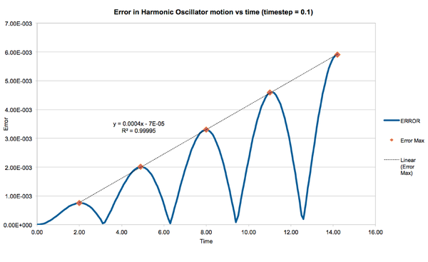
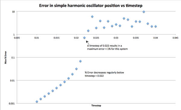
As an exercise, the motion of simple harmonic oscillator was modelled using the Velocity Verlet algorithm for 142 timesteps, for different timestep lengths. The maximum error between the simulated and analytical results was found to increase linearly with time. The maximum error per run decreased as timestep length decreased as expected, and timesteps of length <= 0.022 resulted in errors <1% (figure).

Atomic Forces

Molecular simulations often involve dozens, thousands, or even millions of interactions. However, even simulations of millions of atoms do not model systems on a relateable scale for humans. For example, 0.3 zeptolitres of water (3 x 10^-19 mL) contains 10,000 water molecules, and 33.4 sextillion water molecules would be required to simulate just 1 millilitre of water.

At the multi-molecular scale, quantum effects are relatively small, and intermolecular forces can be approximated by equations from classical dynamics. In our simulations, we will be employing the Lennard-Jones Potential, which includes Pauli exclusion (electron-electron repulsion) at small separations, and Van der Waals attraction at larger separations.

U (r^{N}) = \sum_{i}^{N} \sum_{i \neq j}^{N} {4 ϵ (\frac{σ^{12}}{r_{i j}^{12}} - \frac{σ^{6}}{r_{i j}^{6}})}

For a single Lennard-Jones interaction $ϕ (r) = 4 ϵ (\frac{σ^{12}}{r^{12}} - \frac{σ^{6}}{r^{6}})$ , the separation at which the potential energy is zero is $r_{0} = σ$ , and the force at this separation is $F = \frac{24 ϵ}{σ}$ . The equilibrium separation, ie. the separation at which the net force is zero, is $r_{e q} = \sqrt[6]{2} σ$ , and the well depth is $ϕ (r_{e q}) = - ϵ$ .

The convergence of $ϕ (r)$ at large values of $r$ can be demonstrated by integrations of $ϕ (r)$ (assuming here that $σ = ϵ = 1$ ):

$\int_{2 σ}^{\infty} ϕ (r) d r = - 0.0248$

$\int_{2.5 σ}^{\infty} ϕ (r) d r = - 0.0082$

$\int_{3 σ}^{\infty} ϕ (r) d r = - 0.0033$

As implied here, $l i m_{r \to \infty} ϕ (r) = 0$ , and $ϕ (r)$ is already relatively small at $r = 2 σ$ . To save computational power, this distance can be used as a cutoff for $ϕ (r)$ , above which it is assumed that $ϕ (r) = 0$ .

Boundary Conditions

The boundary properties of the simulation box can be defined in three ways:

Fixed Boundary

A fixed boundary does not change with time, and atoms that exceed a fixed boundary are deleted from the simulation.

Periodic Boundary

A periodic boundary transports any molecule that exits the boundary to a corresponding position on the opposite side of the box. For example, an atom at (0.5, 0.5, 0.5) travelling along (0.7, 0.6, 0.2) in a simulation box which runs from (0, 0, 0) to (1, 1, 1) would appear at (0.2, 0.1, 0.7) after the application of periodic boundary conditions.

Shrink-Wrapped Boundary

The shrink-wrapped boundary expands and contracts dynamically to contain all particles in the simulation. This boundary is demonstrated extension simulations.

Reduced Units

Another convention in molecular dynamics simulations is the usage of reduced units instead of SI units. Reduced units are derived from SI units by dividing the quantity by a standard value, which results in magnitudes that are more easily understood.

eg. Reduced distance $r^{*} = \frac{r}{σ}$

For example, the Lennard-Jones cutoff for Argon is 1.088 nm, which in reduced units is simply r*=3.2. A temperature of 180K can be expressed as T*=1.5, and a well depth of 0.997 kJ/mol can be expressed as T*kB.

The LAMMPS Input File

Lattice Initialization

The geometry of LAMMPS systems is defined using the lattice command, where the lattice type and density is given. lattice is also useful for fluid simulations, as an initial lattice of atoms can be melted to give the desired phase. This is the preferred method for fluid initialization, as it initializes the atoms at a fixed separation from each other. If the atoms were initially assigned random positions, atoms may be initialized very close to, or in the same space as each other. This would introduce a huge amount of energy into the system, and would likely alter the desired conditions.

The lattice density is defined after the lattice type. For example, 'lattice sc 0.8' will define a simple cubic lattice of density 0.8. In the output file, the corresponding line is 'lattice spacing in x, y, z = 1.07722, 1.07722, 1.07722', ie. a unit cell of volume 1.25. Since there is one lattice point per unit cell in the simple cubic lattice, the density is 1/1.25 = 0.8, as defined. A face-centered cubic (fcc) lattice with a density of 1.2 would result in a unit cell length of 1.494, as there are four lattice points per unit cell.

Creating Atoms

Atoms are created in the lattice by first defining a region: 'region box block 0 10 0 10 0 10' defines a block region called box that spans from 0 to 10 unit cell lengths in the x, y, and z directions. Then, the region must be created: 'create_box 1 box' creates the region named box and calls it '1'. This will create atoms based on the defined lattice, for example, a 'sc' lattice will result in 1000 atoms being created, while a 'fcc' lattice will result in 4000 atoms.

Atom properties can be set with a variety of commands. For example:

'mass 1 1.0' sets the masses of all atoms of type 1 to 1.0.

'pair_style lj/cut 3.0' defines the Lennard-Jones pair potential, and sets the cutoff to 3 (reduced units).

'pair_coeff * * 1.0 1.0' sets the pairwise coefficients for all pairs of atoms to 1.0 1.0.

Note: like other programming languages, the LAMMPS input script can be simplified by the use of variables. By initializing and referencing a variable instead of writing raw values in multiple locations, we can edit the properties of the system much more easily, as only one line of code needs to be updated when a parameter changes.

Equilibration

In order to determine a suitable timestep for future simulations, several test simulations were run, and the resulting systems were analyzed. 5 simple cubic lattices (density = 0.8, 1000 lattice points, particle mass = 1.0) in a Lennard-Jones potential field (cut-off = 3, pairwise coefficients = 1.0, neighbor skin = 2.0), each with a different timestep (0.001, 0.0025, 0.0075, 0.01, 0.015), was simulated for floor(100/timesteps) timesteps in the microcanonical (NVE) ensemble. Thermodynamic data (total energy, temperature, pressure) was collected every ten timesteps. This data was then plotted against timestep to determine the most suitable timestep for further simulations.

The most suitable timestep was determined according to two criteria: 1. the timestep must be small enough to allow the system to reach thermodynamic equilibrium, and 2. the timestep must be as large as possible to maximise computational efficiency. Based on these criteria, a timestep of 0.0025 was chosen, as it was the largest timestep with which equilibration was observed. Notably, a timestep of 0.015 did not allow the system to reach equilibrium at all, as seen by the diverging energy.

Thermodynamic variables wrt time for the 0.001 timestep. The system reaches equilibrium at around t=0.15, characterised by constant pressure, temperature, and energy of the system.

Plotting Equations of State

Aim

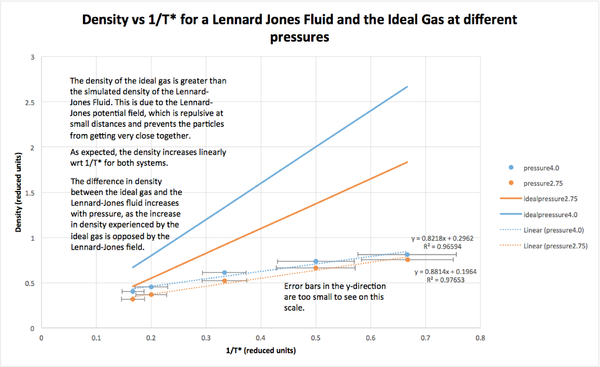
We can determine the equation of state for a Lennard-Jones fluid by monitoring a system's thermodynamic quantities, and plotting them to reveal trends. Here, we expect the density of the system ( $ρ$ ) to increase linearly with $\frac{1}{T}$ . We can confirm this by simulating systems at different fixed pressures and temperatures, and plotting $ρ$ as a function of $\frac{1}{T}$ .

Thermostatting/Barostatting

Fixing thermodynamic variables in LAMMPS is straightforward. The fix command allows you to fix an ensemble, as well as the constants for that ensemble. For example, 'fix npt all npt temp ${T} ${T} ${tdamp} iso ${p} ${p} ${pdamp}' will fix the NPT ensemble with beginning and ending temperatures of 'T', and beginning and ending pressures of 'p'. 'tdamp' and 'pdamp' are the temperature damping parameters, and 'iso' couples all dimensions of the simulation together.

Thermostatting works by using the equipartition principle, which states that the total kinetic energy of a system with three degrees of freedom is equal to $\frac{3}{2} k B T$ . The total kinetic energy $\frac{1}{2} \sum_{i} m_{i} v_{i}^{2}$ is calculated at each step, and compared to $\frac{3}{2} k B 𝔗$ , where $𝔗$ is the target temperature. At each step, the velocities of the particles are multiplied by a scaling factor $γ = \sqrt{\frac{𝔗}{T}}$ to maintain a constant temperature $T = 𝔗$ .

Simulations

Ten simple cubic lattices (density = 0.8, 15x15x15, particle mass = 1.0) in a Lennard-Jones Field (cutoff = 3.0, pair coefficients = 1.0, 1.0) were initialized in the NVE ensemble, each at a different pressure and temperature (pressure = 2.75: temperature = 1.5, 2.0, 3.0, 5.0, 6.0, pressure = 4.0: temperature = 1.5, 2.0, 3.0, 5.0, 6.0). Each simulation was run for 100,000 timesteps (timestep = 0.0025), and thermodynamic data was collected every 10 timesteps. Thermodynamic averages were calculated using the command 'fix aves all ave/time 100 1000 100000 v_dens v_temp v_press v_dens2 v_temp2 v_press2', where '100' how often values are sampled for the averages (ie. every 100 timesteps), '1000' denotes the number of times each sampled value is used to calculate the average, and 100,000 is how often the averages are calculated (ie. every 100,000 timesteps).

The averaged thermodynamic variables were compared to theoretical results for the ideal gas. Upon analysis, it was found that while the expected linear relationship between $ρ$ and $\frac{1}{T}$ was found for all systems, the Lennard-Jones systems had significantly lower densities than the ideal gas, and this difference increased with pressure. This can be attributed to the repulsive Pauli forces in the Lennard-Jones field, which prevent the particles from getting very close to each other. As the ideal gas experiences no such repulsion, its density increases freely with pressure.

Calculating the Heat Capacity

Heat Capacity vs the Variance in Energy

We can use the thermodynamic data collected during simulations to determine useful attributes of the system. For example, the heat capacity of a system is related to the fluctuation in energies by: $C_{V} = \frac{\partial E}{\partial T} = \frac{V a r [E]}{k_{B} T^{2}} = N^{2} \frac{⟨ E^{2} ⟩ - {⟨ E ⟩}^{2}}{k_{B} T^{2}}$ .

Simulations

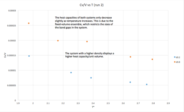
Ten simple cubic lattices (15 x 15 x 15, particle mass = 1.0) in a Lennard-Jones field (cutoff = 3.0, pairwise coefficients = 1,0, 1.0) were initialized in the NVE ensemble, each with a different density and temperature (density = 0.2: temperature = 2.0, 2.2, 2.4, 2.6, 2.8, density = 0.8: temperature = 2.0, 2.2, 2.4, 2.6, 2.8). Simulations were run for 100,000 timesteps (timestep = 0.025), and thermodynamic data every 100 timesteps was averaged to determine the heat capacity of the system.

The calculated heat capacity was divided by the volume of the simulation cell, and plotted against temperature. The resulting data shows an inverse correlation between heat capacity and temperature. This trend is explained by the increasing gap between the ground and excited states as temperature increases. In a fixed volume system, this increase is quite small, and the overall decrease in heat capacity is relatively small.

File:Cv ex input sn3215.in

Finding the Radial Distribution Function

RDF

The radial distribution function is a correlation function for order in a material. If there is a high degree of ordering at a certain distance r, ie. if there is a high probability of finding an atom at a radius of r way from the origin, the RDF will exhibit a peak. The sharpness of the peak can indicate the specificity of this ordering. For example, sharp peaks indicate a crystal-like structure in which the atom spacing is very well-defined. In contrast, a RDF with broad peaks might indicate a liquid or gaseous system, in which there is little to no long-range order.

Simulations

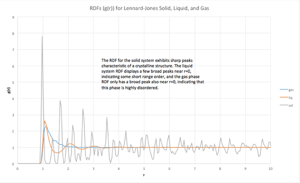
The RDFs of one solid, one liquid and one gaseous Lennard-Jones material were analyzed. The gaseous and liquid simulations were initialized in simple cubic lattices (density = 0.005 and 0.8 respectively, 15x15x15) with temperatures of T=1.0, particles masses = 1.0, and L-J cutoff = 3.2. The solid material was initialized in a face-centered cubic lattice (density = 1.5, 15x15x15) with a temperature T=1.0, particle mass = 1.0, L-J cutoff = 3.2. Each system was simulated for 30,000 timesteps (timestep = 0.002), and the resulting trajectories were analyzed by VMD to extract RDF information.

Phase information was taken from ^[3].

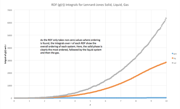
The calculated radial distribution functions matched the expected form for each phase. The solid phase RDF exhibits sharp peaks characteristic of a very ordered material, whereas the liquid and gas RDFs were much broader, with the liquid RDF exhibiting only three broad peaks, and the gas RDF only exhibiting a single broad peak. The overall ordering of each material was quantified by the integral of g(r), which showed that the ordering of the solid was greater than that of the liquid, and gas, and that the gas was the least ordered phase, as expected.

For the solid system, each peak corresponds to a neighboring coordination site. Foe example, the first peak represents the nearest neighbor, the second peak represents the second nearest neighbor, and so on. In a face-centered cubic lattice, the first three nearest neighbors are at r=0.975, 1.375, and 1.675, which correspond to lattice vectors of: (0.5, 0.5, 0) (12-coordinate), (1, 0, 0) (6-coordinate), and (1, 0.5, 0.5) (24-coordinate).

Calculating the Diffusion Coefficient

The diffusion coefficient of a material can be obtained through either of two correlation functions: the mean squared displacement (MSD), and the velocity auctocorrelation function (VACF). These functions are related to the number of collisions a particle in the system experiences, as collisions destroy correlation between positions or velocities.

Simulations

One solid-phase (density = 1.5), liquid-phase (density = 0.8) and gas-phase (density = 0.005) simple cubic lattices (20x20x20) were initialized in a Lennard-Jones field (cutoff = 3.2, pairwise coefficients = 1.0, 1.0) in the NVT ensemble (T=1.0). Each simulation was run for 10,000 timesteps (timestep=0.0025), and the MSD and VACFs for each system were calculated using the compute command.

Additional data from 1,000,000 particle systems was pre-simulated, and used for comparison during data analysis.

MSD

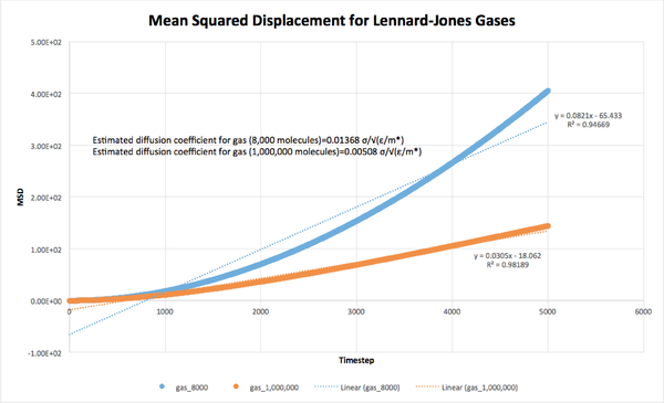
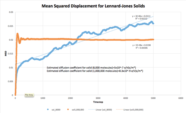
The MSD for each system was plotted against timestep, and the diffusion coefficients were estimated from the equation $D = \frac{1}{6} \frac{\partial ⟨ r^{2} (t) ⟩}{\partial t}$ as:

Gas (8,000 molecules): D = 0.01368 σ/√(ε/m*)

Gas (1,000,000 molecules): D = 0.00508 σ/√(ε/m*)

Liquid (8,000 molecules): D = 1.67*10^-4 σ/√(ε/m*)

Liquid (1,000,00 molecules): D = 1.67*10^-4 σ/√(ε/m*)

Solid (8,000 molecules): D = 5*10^-7 σ/√(ε/m*)

Solid (1,000,000 molecules): D = 8.3*10^-9 σ/√(ε/m*)

As expected, the diffusion coefficient decreased with increasing density of the system, due to the increasing number of collisions occurring at higher densities. Additionally, the larger systems (1,000,000 molecules) all had smaller diffusion coefficients than their smaller counterparts, indicating that the number of collisions in these systems was larger than in the 8,000 molecule systems.

VACF

The Velocity Autocorrelation Function $C (τ) = ⟨ v (t) \cdot v (t + τ) ⟩$ quantifies how different the velocity of an atom will be at time $t + τ$ to time $t$ . We can relate the VACF to the diffusion coefficient by the equation $D = \frac{1}{3} \int_{0}^{\infty} d τ ⟨ v (0) \cdot v (τ) ⟩$ .

Simple Harmonic Oscillator

The VACF of a simple harmonic oscillator is given by $C (τ) = \frac{\int_{- \infty}^{\infty} v (t) v (t + τ) d t (A)}{\int_{- \infty}^{\infty} v^{2} (t) d t (B)}$ . Given that the motion of a simple harmonic oscillator is governed by $x (t) = A c o s (ω t + ϕ)$ , this equation can be simplified as follows:

1. $v (t) = \frac{\partial x (t)}{\partial t} = - A ω s i n (ω t)$ (Assuming $ϕ = 0$ ).

2. Substitute for (A): $A^{2} ω^{2} \int_{- \infty}^{\infty} s i n (ω t) s i n (ω (t + τ)) d t$

3. Since $s i n (A + B) = s i n (A) c o s (B) + s i n (B) c o s (A)$ : $(A) = A^{2} ω^{2} \int_{- \infty}^{\infty} s i n (ω t) [s i n (ω t) c o s (ω τ) + s i n (ω τ) c o s (ω t)] d t$

4. Simplify: $(A) = A^{2} ω^{2} [\int_{- \infty}^{\infty} s i n (ω t) s i n (ω t) c o s (ω τ) d t (A 1) + \int_{- \infty}^{\infty} s i n (ω t) s i n (ω τ) c o s (ω t) d t (A 2)]$

5. Solve A1: $\int_{- \infty}^{\infty} s i n (ω t) s i n (ω t) c o s (ω τ) d t = c o s (ω τ) \int_{- \infty}^{\infty} s i n^{2} (ω t) d t = c o s (τ) - \frac{1}{2} s i n (2 t) |_{- \infty}^{\infty}$

6. Solve A2: $\int_{- \infty}^{\infty} s i n (ω t) s i n (ω τ) c o s (ω t) d t = s i n (ω τ) \int_{- \infty}^{\infty} s i n (ω t) c o s (ω t) = s i n (ω τ) [- \frac{1}{2} c o s^{2} (ω t) |_{- \infty}^{\infty}]$

7. Solve (B): $(B) = A^{2} ω^{2} \int_{- \infty}^{\infty} s i n^{2} (ω t) d t = - \frac{A^{2} ω^{2}}{2} s i n (2 t) |_{- \infty}^{\infty}$

8. Recombine and cancel: $s i n (ω t) |_{- \infty}^{\infty} = 2 s i n (\infty), c o s (ω t) |_{- \infty}^{\infty} = 0$

To find that: $C (τ) = c o s (ω τ)$

Results

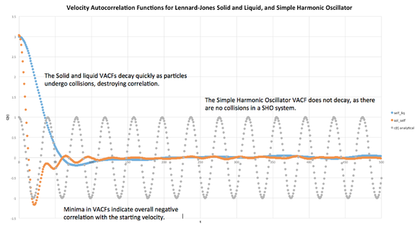
The plotted liquid and solid VACFs were very different from the simple harmonic oscillator VACF, as was expected. This difference is due to the lack of collisions in the simple harmonic oscillator system, ie. its velocity can be predicted at any $τ$ . In contrast, the solid and liquid system VACFs decay very quickly to a minimum, where the overall velocity is negatively correlated to the initial velocity. This indicates that all the particles in the system have undergone collisions. The VACFs then decay to zero as further collisions destroy any remaining correlation, leaving the velocity at a large time $τ$ uncorrelated to the initial velocity.

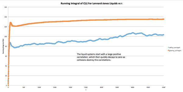
The running integrals of the solid, gas, and liquid systems were plotted, and analysis of the graphs produced the following results:

Solid: The initially high correlation is cancelled out by a corresponding negative correlation, due to the oscillation of atoms about their starting positions. Further collisions then destroy the correlation, leaving the running integral at approximately zero.

Liquid: An initially high correlation is slowly destroyed as collisions occur, but the negative portion of the VCAF does not fully cancel the positive part, leaving a net positive VCAF integral.

Gas: The VCAF integral continues to increase as the simulation is run, due to the low number of collisions in the gas simulation. The larger gas simulation (1,000,000 atoms) shows some asymptotic behavior near the end of the simulation, indicating that collisions have almost destroyed the correlation.

Estimated values of D were calculated using the formula $D = \frac{1}{3} \int_{0}^{\infty} d τ ⟨ v (0) \cdot v (τ) ⟩$ :

Solid (8,000 atoms): 0.023 σ/√(ε/m*)

Solid (1,000,000 atoms): 0.023 σ/√(ε/m*)

Liquid (8,000 atoms): 34.47 σ/√(ε/m*)

Liquid (1,000,000 atoms): 45.05 σ/√(ε/m*)

Gas (8,000 atoms): 4077.7 σ/√(ε/m*)

Gas (1,000,000 atoms): 1634.23 σ/√(ε/m*)

Notably, the larger liquid system displayed a larger diffusion coefficient than the small liquid system. This may be the result of stronger intermolecular structuring in the large system, which would lead to a greater correlation.

As the gaseous systems still displayed positive correlation at the end of the simulation, the diffusion coefficients for these systems could be more accurately with a longer simulation time that allowed the systems to equilibrate fully.

Extension

Simulations of multi-phase systems are very common in research, and can provide information about the dynamics of interfaces and phase boundaries ^[4]. As a further investigation, the dynamics of a liquid bilayer were simulated and analyzed under various conditions.

Note: All trajectories can be visualized using VMD, and atom types can be distinguished by the ‘type’ label.

Experiment 1: liquids of different densities (fixed boundary)

Two simple cubic lattices (15x15x15) were initialized adjacent to each other, one with a density d=0.8 and the other with a density d=0.2, in an NVT ensemble (T=0.5). Particles of mass = 1.0 were created in each lattice, and a Lennard-Jones field was applied (cutoff=3.0, pairwise coefficients = 1.0, 1.0). Fixed boundary conditions were employed, as particle movement through the boundary would result in undesired bypassing of the bilayer interface. The simulation was run for 10,00 timesteps (timestep = 0.0025), and the resulting trajectory was recorded (Ext_35.lammpstrj).

Note: particles occasionally escaped the fixed boundary, which resulted in their removal from the simulation. This would normally raise an error and terminate the simulation, but this was bypassed in this case using ‘thermo_modify lost warn’, which raised an error message when atoms were lost, but allowed the simulation to continue.

Input file: File:Ext 35 sn3215.in

Output: File:Ext 35 output sn3215.txt

Trajectory: emailed to Ollie

Experiment 2: liquids of different densities (shrink-wrapped boundary)

The same lattices and conditions as experiment 1 were used to generate and simulate a liquid bilayer. In this case however, shrink-wrapped boundaries were used to prevent particle deletion. Whereas experiment 1 represented two liquids in a solid container, this experiment more closely models two macromolecules (eg. colloids) interacting in a solvent, as particles are free to move in any direction.

Input file: File:Ext 35 sss sn3215.in

Output: File:Ext 35 sss output sn3215.txt

Trajectory: emailed to Ollie

Experiment 3: liquids of different mass (shrink-wrapped boundary)

A single simple cubic lattice (density = 0.8) was initialized, with type A particles (mass = 1.0) generated in one half, and type B particles mass = 2.0) initialized in the adjacent half. The system was simulated for 10,000 timesteps (timestep = 0.0025) in a Lennard-Jones field in the NVT ensemble with the same conditions as experiments 1 and 2. The resulting trajectory can be visualized in the same way as trajectories from experiments 1 and 2.

In each experiment, some particles tended to move away from the initialized bulk, either being deleted (expt 1) or stretching the boundary and gradually moving further away (expts 2 and 3). However, the majority of the particles stayed within the bulk, and gradual mixing between the layers was observed for each system. Importantly, these systems were simulated at T=0.5, well below the critical temperature. At higher temperatures, it might be expected that a larger percentage, if not all of the particles would diffuse away from the bulk, due to higher kinetic energies resulting in gas-like behavior.

Input file: File:Ext 35 mass sn3215.in

Output: File:Ext 35 mass output sn3215.txt

Trajectory: emailed to Ollie

Further Work

Additional analysis of these systems would potentially involve characterization of the interface between the layers, and analysis of dynamic changes in the density, mass, or other thermodynamic variables at the interface. The method for defining interfaces can also be extended to simulate phase boundaries (eg. solid-liquid), or boundaries between more complex substances (eg. water-oil).

References

↑ J. Phys Chem C, 2016, 120 (30), pp 17035–17045
↑ Lipkowitz, K.B, Cundari, T.R. Reviews in Computational Chemistry, Volume 51, p481
↑ Phys rev. 184, 151, 1969
↑ The Journal of Chemical Physics 68, 3713 (1978); https://doi.org/10.1063/1.436229

[1] J. Phys Chem C, 2016, 120 (30), pp 17035–17045

[2] Lipkowitz, K.B, Cundari, T.R. Reviews in Computational Chemistry, Volume 51, p481

[3] Phys rev. 184, 151, 1969

[4] The Journal of Chemical Physics 68, 3713 (1978); https://doi.org/10.1063/1.436229

[1]

[2]

[3]

[4]