TASK: Open the file HO.xls. In it, the velocity-Verlet algorithm is used to model the behaviour of a classical harmonic oscillator. Complete the three columns "ANALYTICAL", "ERROR", and "ENERGY": "ANALYTICAL" should contain the value of the classical solution for the position at time , "ERROR" should contain the absolute difference between "ANALYTICAL" and the velocity-Verlet solution (i.e. ERROR should always be positive -- make sure you leave the half step rows blank!), and "ENERGY" should contain the total energy of the oscillator for the velocity-Verlet solution. Remember that the position of a classical harmonic oscillator is given by (the values of , , and are worked out for you in the sheet).
TASK: For the default timestep value, 0.1, estimate the positions of the maxima in the ERROR column as a function of time. Make a plot showing these values as a function of time, and fit an appropriate function to the data.
TASK: Experiment with different values of the timestep. What sort of a timestep do you need to use to ensure that the total energy does not change by more than 1% over the course of your "simulation"? Why do you think it is important to monitor the total energy of a physical system when modelling its behaviour numerically?
TASK: For a single Lennard-Jones interaction, , find the separation, , at which the potential energy is zero. What is the force at this separation? Find the equilibrium separation, , and work out the well depth (). Evaluate the integrals , , and when .
TASK: Estimate the number of water molecules in 1ml of water under standard conditions. Estimate the volume of water molecules under standard conditions.
Standard conditions (ambient) = T = 298.15K, P = 1 bar
1mL of water = 1g of water = 1/18 *(6.02 * 10^23) molecules of water = 3.34*10^22 molecules of water
10,000 molecules of water = 10,000/(6.02 * 10^23)*18 grams of water = 10,000/(6.02 * 10^23)*18 mL of water = 3*10^-19 mL of water
TASK: Consider an atom at position in a cubic simulation box which runs from to . In a single timestep, it moves along the vector . At what point does it end up, after the periodic boundary conditions have been applied?.
(0.2, 0.1, 0.7)
TASK: The Lennard-Jones parameters for argon are . If the LJ cutoff is , what is it in real units? What is the well depth in ? What is the reduced temperature in real units?
sigma = 0.34 nm, epsilon/Kb = 120 K, r* = 3.2,
r* in real units = r/sigma, r= sigma*(r*) = 1.088 nm
T* = 1.5 in real units = KbT/epsilon, T = epsilon*(T*)/Kb = 180 K
TASK: Why do you think giving atoms random starting coordinates causes problems in simulations? Hint: what happens if two atoms happen to be generated close together?
- TASK: Satisfy yourself that this lattice spacing corresponds to a number density of lattice points of 1.2
- density of lattice points = lattice points per unit cell/unit cell volume = 1/1.07722^3 = 0.8
. Consider instead a face-centred cubic lattice with a lattice point number density of 1.2. What is the side length of the cubic unit cell?
cell length = 3rt(cell volume) = 3rt(lattice points per unit cell/density of lattice points) = 3rt(4/1.2) = 1.494
TASK: Consider again the face-centred cubic lattice from the previous task. How many atoms would be created by the create_atoms command if you had defined that lattice instead?
1000 unit cells * 4 lattice points per unit cell = 4000 lattice points = 4000 atoms
TASK: Using the LAMMPS manual, find the purpose of the following commands in the input script:
Mass 1 1.0 -> Mass = command for setting atom mass, 1 = atom type, 1.0 = mass
pair_style lj/cut 3.0 -> pair_style = defines pairwise interactions, lj = lennard-jones, cut 3.0 = set cutoff to 3*sigma
pair_coeff * * 1.0 1.0 -> pair_coeff = sets pairwise force field coefficients, * * selects all atoms (otherwise used to set I and J indices), 1.0 1.0 = defined coefficients
TASK: Given that we are specifying xi(0) and vi(0), which integration algorithm are we going to use?
- The Velocity Verlet Algorithm
The second line (starting "variable timestep...") tells LAMMPS that if it encounters the text ${timestep} on a subsequent line, it should replace it by the value given. In this case, the value ${timestep} is always replaced by 0.001. In light of this, what do you think the purpose of these lines is? Why not just write:
- By initializing and referencing a variable instead of writing raw values in multiple locations, we can edit the properties of the system much more easily, as only one line of code needs to be updated when a parameter changes.
Solve these to determine .
gamma=sqrt(squiggleT/T)
TASK: Use the manual page to find out the importance of the three numbers 100 1000 100000. How often will values of the temperature, etc., be sampled for the average? How many measurements contribute to the average? Looking to the following line, how much time will you simulate?
100 = Nevery=take values for average every this many timesteps
1000 = Nrepeat = number of times to use each value to calculate average
10,000 = Nfreq = calculate averages every this many timesteps.
Abstract
Introduction
- Ensemble theory
- Microcanonical (NVE) ensemble was used for timestep determination, isobaric-isothermal(NpT) was used for all other simulations.
Aims and Objectives
Methods
- Initial parameters
- Force field (Lennard-Jones)
- Ideal timestep
- Ideal Gas vs simulation density vs t
- cv/v vs t
- RDFs
Results and Discussion
Conclusion
References
Experimental subsections
- Running your first simulation
Simulations were run on Imperial's High Performance Computing systems using the LAMMPS software package
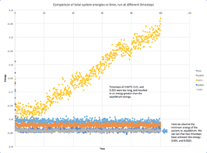
5 simple cubic lattices (density = 0.8, 1000 lattice points, particle mass = 1.0) in a Lennard-Jones potential field (cut-off = 3, pairwise coefficients = 1.0, neighbor skin = 2.0), each with a different timestep (0.001, 0.0025, 0.0075, 0.01, 0.015), was simulated for floor(100/timesteps) timesteps in the microcanonical (NVE) ensemble. Thermodynamic data (total energy, temperature, pressure) was collected every ten timesteps. This data was then plotted against timestep to determine the most suitable timestep for further simulations.
The most suitable timestep was determined according to two criteria: 1. the timestep must be small enough to allow the system to reach thermodynamic equilibrium, and 2. the timestep must be as large as possible to maximise computational efficiency. Based on these criteria, a timestep of 0.0025 was chosen, as it was the largest timestep with which equilibration was observed. Graph used to determine a suitable timestep. The chosen timestep was 0.0025, as it was the longest timestep with which the system achieved equilibrium.
- Introduction to Molecular Dynamics Simulations
TASKS
- Equilibration
Thermodynamic variables wrt time for the 0.001 timestep. The system reaches equilibrium at around t=0.15, characterised by constant pressure, temperature, and energy of the system.TASKS
- Running Simulations under Specific Conditions
THEORY
equipartition theorem: every degree of freedom in a system at equilibrium will have 1/2 KbT of energy. For our system of N atoms and three degrees of freedom, sum(1/2mv^2) = total energy = 3/2NKbT.
- Calculating Heat Capacities Using Statistical Physics
- Structural Properties and the Radial Distribution Function
- Dynamical Properties and the Diffusion Coefficient
Linear trendlines for each phase used to estimate Diffusion Coefficient: