Rep:Sm ising
Ising Model Report - Sam Macer
The Ising model, energy and magnetisation
The Ising model is a simple model which examines the magnetic phase behaviour of a system. The system is set up as an n-dimensional lattice of particles which are either spin up (+1) or spin down (-1). The interaction between any two particles that share a face is counted as an additive contribution towards the overall energy of the system. Each interaction is calculated by multiplying the two spins and then multiplying by some constant J to convert units to energy.
Task 1:
In a lowest energy configuration, all spins will be oriented in the same direction (+1 or -1) to maximise the magnitude of the sum or the interacting spin pairs.
Per dimension, there are two directions in which each spin can interact given that only neighbours sharing a face can interact (modelling the spins as cubes, weather arranged in a line, plane or box).
This means per particle there are 2D interactions, where D = number of dimensions in the system.
The total number of interactions is therefore 2DN/2, where we divide by 2 as each interaction is double counted when we sum interactions over all the particles, where N = number of particles in the system.
Weather each interaction is -1 with -1 or 1 with 1, the magnitude will always be 1, so the total magnitude of the energy of all the interactions will be J * 1.0 * number of interactions where J is some constant converting the units of the energy from arbitrary units into joules.
This simplifies to: Magnitude of the energy of all interactions = DNJ. We know the energy is negative as all spins in alignment correponds to the greatest energy reduction for the system, so we may conclude:
Lowest possible interaction energy for a system (E) = -DNJ
Only two configurations give this state: when either all spins are +1 or all spins are -1.
The multiplicity is therefore given by 2 * N!/N! (= 2) where N is the number of spins in the system.
Entropy (S) = k ln(M) where k is the Boltzmann constant and M is the number of equivalent microstates, so the lowest entropy of the Ising system is given by:
S = k ln(2)
Task 2:
From the lowest energy configuration, if one of the spins were to instantaneously flip, the new configuration would be all spins aligned but one; i.e all +1 with one -1 or all -1 with one +1.
Multiplicity therefore = 2 * N!/(N - 1)!
The entropy for the D =3, N =1000 system is therefore k ln(2 * (1000!/999!))
S = k ln(2 * (1000!/999!))
S = k ln(2000)
In terms of the energy, one spin interacts with 6 neighbours in a 3D lattice. One positive interaction changing into one negative interaction increases the energy by 2J, so overall, flipping one spin leads to a 12J increase in energy to the system.
Magnetisation
The magnetisation of the system is defined as the sum of all the spins in the system.
Task 3:
System 1:
+ + + - -
For system 1, the total magnetisation is 3 - 2:
Magnetisation = + 1
System 1:
+ + + + -
+ + + - -
+ + + - -
+ + - - -
+ - - - -
For system 1, the total magnetisation is 13 - 12:
Magnetisation = + 1
At absolute zero the entropic contribution would be minimised, so one would expect the energetic contribution to dominate and align all the spins.
At absolute zero therefore, for a 3D system of 1000 spins, magnetisation = 1000
Python (Energy and magnetisation)
Task 4
Functions to extract the energy and magnetisation of a system were then written in python;
   def energy(self):
       "Return the total energy of the current lattice configuration."
       # Function works by cycling through each element and then interacting with each neighbour on a grid of coordinates. The energy is halved to prevent double counting and made negative.
       energy = 0.0
       net_interaction = 0
       y = 0
       x = 0
       for row in self.lattice:
               for element in row:
                   # interact right
                   if x != self.n_cols - 1:
                       net_interaction += (element * self.lattice[y, x + 1])
                   else:
                       # if we are at the end element, interact with the adjacent system
                       net_interaction += (element * self.lattice[y, 0])
                   # interact left
                   if x != 0:
                       net_interaction += (element * self.lattice[y, x - 1])
                   else:
                       # if we are at the start element, interact with the adjacent system
                       net_interaction += (element * self.lattice[y, self.n_cols - 1])
                   # interact bottom
                   if y != self.n_rows - 1:
                       net_interaction += (element * self.lattice[y + 1, x])
                   else:
                       # if we are at the end element, interact with the adjacent system
                       net_interaction += (element * self.lattice[0, x])
                   # interact top
                   if y != 0:
                       net_interaction += (element * self.lattice[y - 1, x])
                   else:
                       # if we are at the start element, interact with the adjacent system
                       net_interaction += (element * self.lattice[self.n_rows - 1, x])
                   # iterate selected spin
                   if x == self.n_cols - 1:
                       x = 0
                       y += 1
                   else:
                       x += 1
       interaction_energy = - 0.5 * net_interaction
       return interaction_energy
   def magnetisation(self):
       "Return the total magnetisation of the current lattice configuration."
       magnetisation = 0
       for row in self.lattice:
           for element in row:
               magnetisation += element
       return magnetisation
Task 5
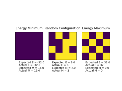
The 'ILcheck.py' script was then ran multiple times to check the energy and magnetisation functions gave consistently correct results:
Python (Monte Carlo Function)
Task 6
Let us consider a system with 100 spins. Considering each spin has two possible states, there are potential configurations of the system. Even if we could analyse configurations per second, it would still take us to calculate the magnetisations of all of the configurations to take an average. Clearly this would take too long so we must look for an alternative method of gathering data on the behaviour of the energy. One way of doing this is using a Monte Carlo simulation where we start with a random configuration and randomly flip spins. We accept the new configuration if there is an energy reduction. Otherwise we accept the new configuration at a rate proportional to the Boltzmann factor as this reflects how often a particle would theoretically have enough energy to flip to a higher energy state.
Task 7
A Monte-Carlo simulation was coded in python as follows:
   def montecarlostep(self, T):
       "preforms a single Monte Carlo step"
       energy = self.energy()
       current_lattice = self.lattice
       # create a new lattice with on spin flipped
           #the following two lines select the coordinates of the random spin
       random_i = np.random.choice(range(self.n_rows))
       random_j = np.random.choice(range(self.n_cols))
       self.lattice[random_i][random_j] =  -self.lattice[random_i][random_j]
       new_E = self.energy()
       # compare energies and decided what configuration to adopt, then update parameters
       dE = new_E - energy
       if dE < 0:
           # print('new energy lower: lattice updated')
           pass
       else:
           # the following line will choose a random number in the range (0,1)
           randNumb = np.random.random()
           if randNumb <= math.exp(-dE/T):
               # print('lattice was updated')
               pass
           else:
               # print('lattice was not updated')
               self.lattice[random_i][random_j] =  -self.lattice[random_i][random_j]
       self.E += self.energy()
       self.E2 += self.energy()**2
       self.M += self.magnetisation()
       self.M2 += self.magnetisation()**2
       # converts cycle index x to cycle number x + 1 (the next machine cycle step number)
       # In other words increments the counter of number of cycles
       self.n_cycles += 1
       return self.energy(), self.magnetisation()
   def statistics(self):
       "returns statistical data collected during a Monte Carlo simulation"
       avE = self.E / self.n_cycles
       avE2 = self.E2 / self.n_cycles
       avM = self.M / self.n_cycles
       avM2 = self.M2 / self.n_cycles
       N = self.n_cycles
       return avE, avE2, avM, avM2, N
Task 8
When the temperature of the system is above the Curie Temperature (Tc), the system is paramagnetic at thermodynamic equilibrium, i.e. the spins are oriented randomly in the absence of an external magnetic field. When the temperature of the system is below the Curie Temperature, the system is ferromagnetic at thermodynamic equilibrium (spins align). In the case T < Tc, one would therefore expect the system to spontaneously magnetise (spins align) as it attains the most thermodynamically stable state.
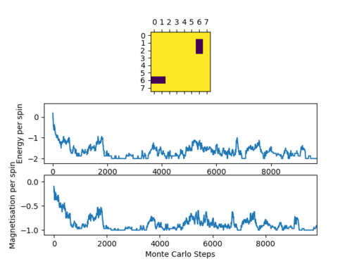
Indeed, when we run our Monte Carlo simulation for an 8x8 lattice at T = 0.5 K, it can be seen that the spins tend toward alignment in on direction as the energy minimises;
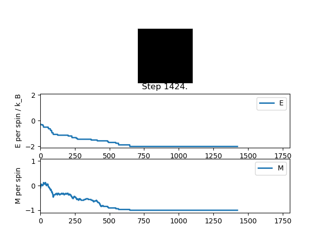
   Averaged quantities:
   E =  -1.96841896186
   E*E =  3.88120282707
   M =  -0.991326800847
   M*M =  0.983257746292
Accelerating the code
Task 9
In an attempt to accelerate the code and save time, the energy() and magnetisation() functions were made more efficient using functions within the numpy python library:
   def energy(self):
       "Improved energy function which implements numpy's roll and multiply functions"
       # multiply by a shifted grid to apply vertical energy contribution
       vertical_energy = -np.sum(np.multiply(self.lattice, np.roll(self.lattice, 1, axis = 0)))
       # multiply by a shifted grid to apply the horizontal energy contribution
       total_energy = vertical_energy - np.sum(np.multiply(self.lattice, np.roll(self.lattice, 1, axis = 1)))
       return total_energy
   def magnetisation(self):
       "Improved magnetisation function that implements numpy's sum function:"
       return np.sum(self.lattice)
Task 10
Time trials were used to compare the speed of the old and updated energy functions:
   New function:
   2.4918089999999893 s
   2.4761589999999956 s
   2.540256999999997 s
   2.4700420000000065 s
   2.5968489999999917 s

   Average = 2.52 s
   Standard error of average = 0.024 s

   Old function:
   10.844294 s
   10.496529000000002 s
   10.151754999999998 s
   10.489855999999996 s
   9.988599999999998 s

   Average = 10.39 s
   Standard error of average = 0.149 s
The result is the improved function only takes 24.3 % of the time took by the old function to do the same thing.
The effect of temperature
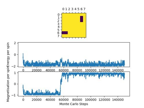
The following plots were produced by running 150000 steps of the Monte Carlo simulation at T = 0.5 K and T = 2.0 K respectively:
Note, in the second system, we see that there must be a realistic chance for the whole system to flip the net spin direction as this is what can be seen from the graph to occur. This happens because in this system there are two global minimum points on the potential energy surface separated by a barrier. At this temperature there is enough energy to only occasionally overcome this barrier.
Task 11
Looking at the dynamics of the systems, we can see in the temperature region in which we are working, the region after 3000 steps should be a sufficient representation of the system at equilibrium. The Monte Carlo step and statistics functions were updated to only begin the statistics functionality after 3000 steps:
   # Defines first cycle in which statistical data is collected
   statsStartStep = 3000
   # Converts cycle nummber into the machine read index of the cycle (humans count from 1, machine indexes from 0)
   statsStartStep -= 1
   def montecarlostep(self, T):
       "preforms a single Monte Carlo step"
       energy = self.energy()
       current_lattice = self.lattice
       # create a new lattice with on spin flipped
           #the following two lines select the coordinates of the random spin
       random_i = np.random.choice(range(self.n_rows))
       random_j = np.random.choice(range(self.n_cols))
       self.lattice[random_i][random_j] =  -self.lattice[random_i][random_j]
       new_E = self.energy()
       # compare energies and decided what configuration to adopt, then update parameters
       dE = new_E - energy
       if dE < 0:
           # print('new energy lower: lattice updated')
           pass
       else:
           # the following line will choose a random number in the range (0,1)
           randNumb = np.random.random()
           if randNumb <= math.exp(-dE/T):
               # print('lattice was updated')
               pass
           else:
               # print('lattice was not updated')
               self.lattice[random_i][random_j] =  -self.lattice[random_i][random_j]
       # Update the running total IF we are in the region we are gathering stats for
       if self.n_cycles >= self.statsStartStep:
           self.E += self.energy()
           self.E2 += self.energy()**2
           self.M += self.magnetisation()
           self.M2 += self.magnetisation()**2
       # converts cycle index x to cycle number x + 1 (the next machine cycle step number)
       self.n_cycles += 1
       # print(self.n_cycles)
       return self.energy(), self.magnetisation()
   def statistics(self):
       # Updated statistics function
       if self.n_cycles >= self.statsStartStep:
           avE = self.E / (self.n_cycles - self.statsStartStep)
           avE2 = self.E2 / (self.n_cycles - self.statsStartStep)
           avM = self.M / (self.n_cycles - self.statsStartStep)
           avM2 = self.M2 / (self.n_cycles - self.statsStartStep)
           N = self.n_cycles
       return avE, avE2, avM, avM2, N
The effect of system size
Task 12
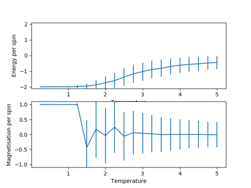
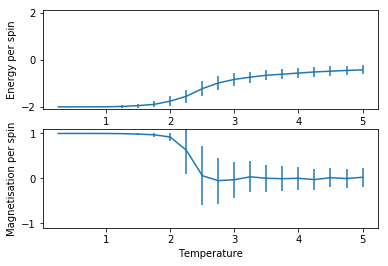
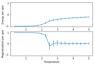
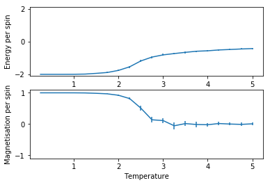
A function was then used to plot average energy per spin and average magnetisation per spin against temperature from T = 0.25 K to T = 5 K in 0.25 K intervals. Error bars represent one standard deviation's worth of uncertainty for the calculation. This was done for 2x2, 4x4, 8x8, 16x16 and 32x32 size lattices, graphed in the same order:
2x2
4x4
8x8
16x16
32x32
All of the graphs show a convergence to a limiting value at high temperatures showing the Temperature a) ceases to affect magnetisation (the paramagnetic state) and b) subsequently ceases to affect energy stabilisation due to spin alignment (there are no more static alignment effects). The magnetisation graphs show an oscillating convergence because the spin of the hole system can flip near the Curie temperature as explained earlier. Both +1 and -1 spin systems provide the same energy stabilisation to the system, so energy does not oscillate in it's convergence.
The error bars for both quantities peak around the Curie temperate presumably as at this point the system is most often undergoing full system spin flips, causing a large variance. At the beginning of the plot the variance is low as expected because there is little dynamic activity. At the end of the plot, even though there is a lot of noise and hence wild oscillation of the spins in the system, there is so much energy that almost any change is accepted, and so the extreme configurations (i.e. all aligned) rarely occur because statistically they are so unlikely to occur. This means the variation in energy and magnetisation for the most part varies within a smaller range and so the errorbars of one standard deviation (95% confidence) are smaller.
The variation between the plots themselves can also be elucidated:
Task 13
The average energy per spin plots were superimposed. What we see is the convergence of the energy to a certain curve for large lattices:
This shows the lattice size is large enough to properly model long range effects as increasing the lattice size has little further effect.
The plot superimposing the magnetisations is also interesting. Firstly we see the magnitude of magnetisation per spin is pretty constant which is exactly what we would expect. Secondly we can see the oscillating convergence much more clearly. Finally we see the convergence is quickest for the smaller lattices, presumably because it's much easier kinetically to have an even distribution of spins.
Determining the heat capacity (C)
Task 14
We know the average energy is equal to the probability of each energy times the energy. In terms of the partition function (Z, Statistical thermodynamics), we can write this and rearrange to get: .
Considering , we can rearrange (by equating the squared average energy in both equations) to:
Using (The defenition of heat capacity):
We obtain via integration:
Task 15
Heat capacity can therefore be worked out using;
   x2 = np.array(np.loadtxt('2x2.dat'))
   varEx2 = x2[:,2]-x2[:,1]**2
   cx2 = varEx2 / x2[:,0]**2
   # Plot and make the heat capacity per spin by dividing by lattice size
   pl.plot(x2[:,0], cx2/4, color = 'green')
for each lattice size, where 2x2.dat is a table with columns [Temperature, Average energy, Average squared energy, Average Magnetisation, Average Squared Magnetisation]. After running each simulation 5 times and then averaging for more accurate data, the Heat capacity per spin was subsequently plotted as a function of temperature and lattice size:
The plot shows that as you increase the lattice size, there is a tighter convergence to some central peak, which implies an infinite lattice would contain a sharp, infinite peak. This is characteristic of a first order phase transition. Based on the observed behaviour of our spins, this phase transition would be the ferromagnetic - paramagnetic phase transition at the Curie temperature.
Finding the Curie temperature (Tc)
Task 17
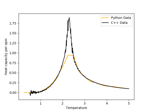
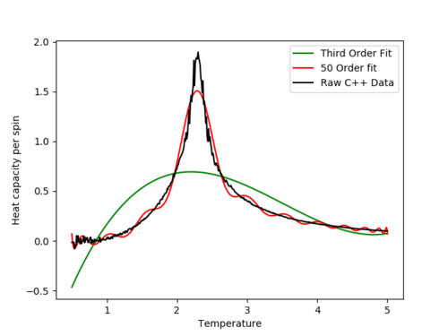
A set of data ranging from 2x2 to 64x64 lattices using a more advanced simulation written in C++ was provided. This data was plotted and compared to the data from this experiment. An example plot is shown (for the 32x32 lattice size). The C++ data exhibits a much taller and sharper peak. This may be partially down to the low (T = 0.25 K spacing) resolution of the python data (which could be resolved better given more time). The non-peak regions match well which suggests that overall the experimental method is good.
Task 18
A plot was then written to fit a polynomial to the C++ data;
   import numpy as np
   import matplotlib.pyplot as pl
   data = np.loadtxt('32x32C.dat') #assume data is now a 2D array containing two columns, T and C
   T = data[:,0] #get the first column
   C = data[:,5] # get the second column
   #first we fit the polynomial to the data
   fit = np.polyfit(T, C, 3) # fit a third order polynomial
   #now we generate interpolated values of the fitted polynomial over the range of our function
   T_min = np.min(T)
   T_max = np.max(T)
   T_range = np.linspace(T_min, T_max, 1000) #generate 1000 evenly spaced points between T_min and T_max
   fitted_C_values = np.polyval(fit, T_range) # use the fit object to generate the corresponding values of C
   pl.plot(T_range, fitted_C_values, color = 'green')
   fit50 = np.polyfit(T, C, 50)
   fitted_C_values50 = np.polyval(fit50, T_range) # use the fit object to generate the corresponding values of C
   pl.plot(T_range, fitted_C_values50, color = 'red')
   x32C = np.array(np.loadtxt('32x32C.dat'))
   pl.plot(x32C[:,0], x32C[:,5], color = 'black')
   pl.ylabel('Heat capacity per spin')
   pl.xlabel('Temperature')
   pl.legend(['Third Order Fit', '50 Order fit', 'Raw C++ Data'])
   pl.show()
The graph shows both the original data, a polynomial fir of order 3 and a polynomial fit of order 50:
Even though using higher order polynomials provides a much more accurate fit, upon increasing the order we get diminishing returns on accurately modelling the peak.
Task 19
As we are mainly interested in finding the Curie temperature, an accurate fit of the peak is most important. An updated plot was executed to fit only in the region around the fit:
   import numpy as np
   import matplotlib.pyplot as pl
   data = np.loadtxt('32x32C.dat') #assume data is now a 2D array containing two columns, T and C
   T = data[:,0] #get the first column
   C = data[:,5] # get the second column
   Tmin = 2.1 #for example
   Tmax = 2.6 #for example
   selection = np.logical_and(T > Tmin, T < Tmax) #choose only those rows where both conditions are true
   peak_T_values = T[selection]
   peak_C_values = C[selection]
   selection = np.logical_and(T > Tmin, T < Tmax) #choose only those rows where both conditions are true
   #first we fit the polynomial to the data
   fit = np.polyfit(peak_T_values, peak_C_values, 3) # fit a third order polynomial
   #now we generate interpolated values of the fitted polynomial over the range of our function
   T_range = np.linspace(Tmin, Tmax, 1000) #generate 1000 evenly spaced points between T_min and T_max
   fitted_C_values = np.polyval(fit, T_range) # use the fit object to generate the corresponding values of C
   pl.plot(T_range, fitted_C_values, color = 'green')
   fit50 = np.polyfit(peak_T_values, peak_C_values, 50)
   fitted_C_values50 = np.polyval(fit50, T_range) # use the fit object to generate the corresponding values of C
   pl.plot(T_range, fitted_C_values50, color = 'red', linestyle='--')
   x32C = np.array(np.loadtxt('32x32C.dat'))
   pl.plot(x32C[:,0], x32C[:,5], color = 'black', linestyle=':')
   pl.ylabel('Heat capacity per spin')
   pl.xlabel('Temperature')
   pl.legend(['Third Order Fit', '50 Order fit', 'Raw C++ Data'])
   pl.show()
The peak was found to be at the [T, C] coordinate: [2.29369369, 1.85691773891] for the 32x32 lattice.
Task 20
The above was then repeated to get the Curie temperature as a function of lattice size:
   Lattice Size Curie Temperature
   2 2.5105105105105103
   4 2.4564564564564564
   8 2.3283283283283285
   16 2.31031031031031
   32 2.293693693693694
   64 2.2732732732732734
It can be shown:
, where is the Curie temperature of an lattice, is the Curie temperature of an infinite lattice, and is some constant.
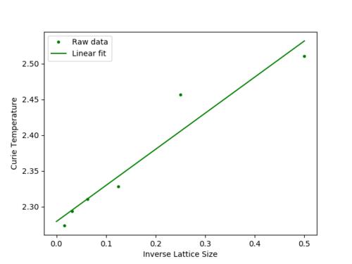
In order to obtain the Curie temperature of an infinite lattice, 1/L was plotted against Tc(L) and a linear fit was performed:
Tc for an infinite lattice is T at the Tc(L) intercept:
The data appears to have a reasonable fit, though there are only 5 data points, so the fit would benefit from using more lattice sizes.
According to the literature, the theoretical Curie temperature for an infinite lattice is Tc = 2.269J (Source: Numerical Methods for Chemical Engineering: Applications in MATLAB By Kenneth J. Beers.) This is only 0.01 away from the fitted result, which shows the experimental data and fitting equation are both fairly accurate.


