Introduction

The Ising lattice model uses statistical thermodynamics to describe many body systems. It is a powerful toy model that captures a variety of physical behaviour, most notably phase transitions and heat capacity's dependence on temperature. Like any general statistical mechanics problem however, solving for properties of the Ising model analytically is non-trivial: any high fidelity simulation will have a large number of interacting bodies and feature many possible combinations. Although contemporary computational methods can calculate properties of a given system configuration rapidly, it is still limited by the sheer number of configurations that need to be evaluated. An alternative computational method, the Monte Carlo (MC) Metropolis-Hastings algorithm ^[1], bypasses the issue by sampling the most representative configurations at a given temperature, negating the requirement to compute all possible states and shortens the otherwise long computational time issue.

In this experiment, the Metropolis-Hastings algorithm was used to find the lowest free energy state of ferromagnetic Ising lattices with different sizes. By:

determining whether the lowest free energy state has any net magnetisation, and
determining how the heat capacity of the lowest free energy state changes

over a range of temperatures, it was possible to locate the critical temperature where the system becomes diamagnetic, the equivalent of the Curie temperature in real physical systems. The behaviour of the simulated system around the critical point was studied.

The MC simulation performance of two programming languages, Python and C++, were compared and contrasted.

The Ising Model

The Model

The Ising model assumes the following ^[2]:

Consider an array of particles each with net magnetic dipole moment of $1$ observing boundary conditions. Each particle in this lattice space $s_{i}$ can take values $+ 1$ or $- 1$ , corresponding to the magnetic dipole moment of 'up' or 'down'.
The interaction energy between adjacent particles $i, j$ is defined as the product of their moments and the interaction strength $J s_{i} s_{j}$ . If $J > 0$ , it is a ferromagnetic interaction; this was the case used in the exercise.
The total interaction energy of a lattice at a certain configuration $α$ is the Hamiltonian $E (α) = - \frac{J}{2} \sum_{i}^{N} \sum_{j \in n (i)} s_{i} s_{j} - μ \sum_{i} B s_{i}$ where $j \in n (i)$ are the neighbours of $i$ , $μ$ is the magnetic moment and $B$ is the external magnetic field. The first term corresponds to neighbouring spin interactions, the last term corresponds to interaction with the external magnetic driving force.
With no external magnetic field, only adjacent magnetic interactions contribute to the aforementioned Hamiltonian, and the second term vanishes. In this exercise no external magnetic field was simulated.

TASK: Show that the lowest possible energy for the Ising model is $E = - D N J$ , where $D$ is the number of dimensions and $N$ is the total number of spins. What is the multiplicity of this state? Calculate its entropy.

In a $1 D$ lattice, each particle has $2$ neighbours; in a $2 D$ lattice, each particle has $4$ neighbours, and so on. Thus in general for a lattice of dimension $D$ the number of neighbours at any position is $2 \times D$ . The interaction energy of a lattice is minimised when all the magnetic moments are parallel ( $s_{i} s_{j} = 1$ for all $s_{i}, s_{j}$ ). Hence:

\sum_{j \in n (i)} s_{i} s_{j} = 2 D

E_{m i n} = - \frac{1}{2} J \sum_{i}^{N} 2 D

∴ E_{m i n} = - N D J

The entropy of a system is given by:

S = k_{B} l n Ω

where $Ω$ is the multiplicity of a lattice configuration:

Ω = \frac{N!}{n_{+ 1}! n_{- 1}!}

The state of an Ising lattice with the lowest internal energy is where all the spins are parallel, and there are two isoenergetic configurations which yield such a result; a lattice with all spins up and one with all spins down. Since each of these configurations have $Ω = 1$ , the lowest energy state of an Ising lattice has multiplicity $Ω = 2$ . The entropy of the system is $S = k_{B} \ln 2$ , consistent with the Third Law of thermodynamics which states that the entropy approaches a constant value as $T \to 0$ ^[3].

Phase Transition

The Ising lattice is one of the simplest model for describing phase transitions.

TASK: Imagine that the system is in the lowest energy configuration. To move to a different state, one of the spins must spontaneously change direction ("flip"). What is the change in energy if this happens ( $D = 3, N = 1000$ )? How much entropy does the system gain by doing so?

Consider a lattice with $D = 3$ and $N = 1000$ at its lowest possible total energy state, with all spin states parallel. The switching of one spin position increases the interaction energy of the entire lattice. The total energy increase is the loss of favourable interactions plus increase in unfavourable interactions. The size of this change can be determined by observing the case presented in Figure 1: in a 3D lattice each lattice position has 6 neighbours. To flip the spin at the lattice position concerned, the interaction energy increase is $6 J$ (for loosing $6$ favourable parallel-spin interactions) plus another $6 J$ (for gaining $6$ antiparllel-spin interactions). The total system interaction energy of the new configuration is thus:

E = - 1000 \times 3 \times J + 12 J = - 2988 J

The multiplicity of the new configuration is $1000 \times 2$ . The entropy is $S = k_{B} \ln 2000$ . Entropy gained by the system when it makes such a transition is thus:

Δ S = k_{B} (\ln 2000 - \ln 2) = k_{B} \ln \frac{2000}{2} = k_{B} \ln 1000

Since the new configuration has a higher total energy, the system must have enough thermal energy to access this state.

As the temperature increases more configurations with anti-parallel spins are accessible, to a point where states with all spins randomised are accessible and there is little regular structure. It is possible to quantify the 'regularity' of an Ising lattice configuration by defining the magnetisation, which is the sum of all the magnetic dipole moments in the lattice:

M = \sum_{i} s_{i}

At low temperatures, the most accessible state has many parallel spins thus large magnetisation, and vice versa.

TASK: Calculate the magnetisation of the 1D and 2D lattices below. What magnetisation would you expect to observe for an Ising lattice with $D = 3, N = 1000$ at absolute zero?

Consider the following systems:

For the depicted $D = 1$ , $N = 5$ system in Figure 2, $M = \pm 1$
For the depicted $D = 3$ , $N = 25$ system Figure 2, $M = \pm 1$
For a system of $D = 3$ , $N = 1000$ , at $T = 0$ , the system only has access to the lowest energy state where all the spins are parallel, thus $M = \pm 1000$

It follows that as the temperature increase and configurations with lower spin 'regularity' are accessed, the magnetisation must decrease then at some point drop to $0$ when the temperature reaches a critical point and the spins are virtually randomised. This critical temperature $T_{c}$ marks the transition between the magnetised phase and non-magnetised phase, and is indeed observed empirically (known as the Curie temperature). The validity of using the Ising model to describe ferromagnetic materials could in part be assessed by how well it replicates such behaviour (an investigation featured in later parts of this laboratory). Criticality of this nature also manifests in other phase transitions such as melting and boiling, presenting a motivation to understand what is happening at these points albeit in a simple model.

Energy and Magnetisation Calculations

To determine properties of an Ising lattice, the object IsingLattice(n_rows, n_cols) was constructed using Python 3.7, which receives the arguments n_rows, n_cols and generates an Ising lattice of n_rows rows by n_cols columns with randomised magnetic moments. It also contains relevant functions that calculate the total interaction energy and magnetisation of a given lattice object.

Modifying the Files

TASK: Complete the functions energy() and magnetisation(), which should return the energy of the lattice and the total magnetisation, respectively. In the energy() function you may assume that $J = 1.0$ at all times. The efficiency of the code will be addressed in a later part of the experiment.

The function energy() in the IsingLattice() object calculates the Hamiltonian of a simulated Ising lattice with a given configuration of spins:

    def energy(self):
        "Returns the total energy of the current lattice configuration."
        row = []
        interactions = 0
        J = 1.0
        for i in range(self.n_rows):
            row = row + [self.lattice[i]*self.lattice[i-1]]
            for j in range(self.n_cols):
                interactions = interactions + self.lattice[i][j]*self.lattice[i][j-1]
        interactions = interactions + np.sum(row)
        energy = interactions * -J
        return energy

The interaction strength parameter was kept for completeness. This process utilised the fact that for each element in a $2 D$ lattice, only $2$ of its $4$ neighbouring interactions need to be accounted for. Under the numpy.array architecture of the lattice object, the vertical and horizontal energy contributions were obtained as such (Figure 3):

each row is multiplied with the row above it to create another matrix of the same size. Sum over all elements to get the vertical contribution.
each element in a row is multiplied by its previous neighbour and the product is combined with the last. Repeat for every element to give the horizontal contribution.

This was not efficient code. The code optimisation is addressed in a later part. The function magnetisation() calculates the total magnetisation for a given configuration in the same simulated Ising lattice:

    def magnetisation(self):
        "Return the total magnetisation of the current lattice configuration."
        magnetisation = np.sum(self.lattice)
        return magnetisation

Here a numpy.sum function over array elements was used.

Testing the Files

TASK: Run the ILcheck.py script from the IPython Qt console using the command

%run ILcheck.py

The displayed window has a series of control buttons in the bottom left, one of which will allow you to export the figure as a PNG image. Save an image of the ILcheck.py output, and include it in your report.

The accompanying checking script ILcheck.py was executed to check that the IsingLattice object behaved as expected. The simulation computed total energies and magnetisations for three configurations as predicted.

Introduction to Monte Carlo Simulation

Average Energy and Magnetisation

Consider an Ising lattice in equilibrium with a heat bath at temperature $T$ . If $T$ is not too low, there are many thermally accessible unique configurations $α$ , each with a different total interaction energy $- E (α)$ . The probability of observing the crystal in a certain spin configuration is given by:

P_{T} (α) = \frac{e^{\frac{- E (α)}{k_{B} T}}}{\sum_{α} e^{\frac{- E (α)}{k_{B} T}}} = \frac{1}{Q} e^{\frac{- E (α)}{k_{B} T}}

where the denominator is the partition function of the canonical ensemble for the Ising lattice at temperature $T$ , describing which of the configurations are accessible at that temperature. The probability of finding the lattice at some energy will have to take degeneracy $g (E)$ into consideration:

P_{T} (E) = \frac{g (E)}{Q} e^{\frac{- E}{k_{B} T}}

The expectation or mean value of a measurable quantity corresponding to the lattice is:

⟨ f ⟩_{T} = \sum_{α} f (α) P_{T} (α)

The expected value of the total system energy is hence:

{⟨ E ⟩}_{T} = \sum_{α} E (α) P_{T} (α) = \frac{1}{Q} \sum_{α} E (α) e^{- \frac{E (α)}{k_{B} T}}

The internal energy of the system at $T$ is equivalent to the average total energy of thermally accessible configurations:

U (T) = {⟨ E ⟩}_{T}

As the system is in equilibrium with the temperature bath, its free energy is at a minimum. The equilibrium structure will therefore have:

a minimised average total energy $⟨ E ⟩$ or internal energy, which will have to feature significant contribution from the lowest total energy state (all spins parallel) for $⟨ E ⟩$ to be truly minimised.
a maximised entropy, which is featured in the fluctuation between thermally accessible energy states. As the temperature increases, more of these states will be accessible.

Another way to characterise the system when it is at equilibrium is to define the average magnetisation over all the thermally accessible configurations around the minimum total energy (at $T$ ):

{⟨ M ⟩}_{T} = \frac{1}{Q} \sum_{α} M (α) e^{- \frac{E (α)}{k_{B} T}}

There is strong incentive to calculate the properties of all possible configurations and use the partition function to scale their respective contributions to the overall measured physical quantity.

TASK: How many configurations are available to a system with 100 spins? To evaluate these expressions, we have to calculate the energy and magnetisation for each of these configurations, then perform the sum. Let's be very, very, generous, and say that we can analyse $1 \times 1 0^{9}$ configurations per second with our computer. How long will it take to evaluate a single value of ${⟨ M ⟩}_{T}$ ?

However to compute the aforementioned properties such as magnetisation for all possible configurations is computationally costly. For a system with $100$ spins, there are $2 \times 100 = 1.27 \times 1 0^{30}$ possible configurations. Assuming $1 0^{9}$ configurations can be computed per second using contemporary methods, it will take $1.27 \times 1 0^{21}$ seconds, which is roughly $40$ trillion years. This is clearly an unjustifiable timescale for a simulation. Smarter methods are required to extract information from the model. Although analytical solutions to the partition function exist for one dimensional and two dimensional Ising lattices, a numerical method was used in this exercise.

Incorporating Monte Carlo Method

The MC Metropolis-Hastings algorithm is a sampling algorithm which randomly navigates, in chained steps, through a many-variable probability distribution and selects the configurations which satisfy a certain probability acceptance threshold. The result is a distribution which should resemble the original.

In this exercise, this algorithm was used to sample through possible configurations that an Ising lattice can take at equilibrium, and the configurations which were most likely accessible around the equilibrium were kept. The expected probability distribution is a Gaussian centred around the lowest energy coniguration (all spins parallel). First an Ising lattice with a random configuration was generated, then the algorithm took its course following the flowchart below:

**Figure 5**: The MC Metropolis-Hastings algorithm.

As evident form the flowchart, the algorithm:

should ultimately seek the configuration with minimum total energy
should fluctuate (depending on temperature) around the minimum, and sample configurations with energies accessible at a given temperature defined by the Boltzmann distribution.

In the process of minimising internal energy and allowing for almost mechanical 'thermal fluctuations' realised by the Metropolis-Hastings algorithm, the free energy is actually minimised. Once the random walk reaches the global minimum, the samples acquired as the thermal fluctuations progress describes the equilibrium structure: the lowest energy states will have the biggest contribution to the sample, but the higher energy states will only occasionally be sampled and thus have less contribution. Since the underlying distribution at equilibrium is a Gaussian centred about the lowest interaction energy configuration, the size of the thermal fluctuations should be of the magnitude $\frac{1}{\sqrt{N}}$ ^[4].

The average total energy of the samples collected around the lowest energy state is roughly the same as the minimum internal energy if it was calculated by partition functions:

⟨ E ⟩_{T} \approx \frac{1}{n} \sum_{n} E (α)

where $n$ is the number of samples acquired. As the number of samples increase the modelled distribution should approach that of the analytical result. The same logic was used to find the expected magnetisation of the sample.

Modifying IsingLattice.py

TASK: Implement a single cycle of the above algorithm in the montecarlocycle(T) function. This function should return the energy of your lattice and the magnetisation at the end of the cycle. You may assume that the energy returned by your energy() function is in units of $k_{B}$ ! Complete the statistics() function. This should return the following quantities whenever it is called: $⟨ E ⟩, ⟨ E^{2} ⟩, ⟨ M ⟩, ⟨ M^{2} ⟩$ , and the number of Monte Carlo steps that have elapsed.

Initially the basic Metropolis-Hastings algorithm was implemented in the IsingLattice object:

    def montecarlostep(self, T):
        "Function performing a single Monte Carlo sampling step. Returns energy and magnetisation sum."
        energy_i = self.energy()
        random_i = np.random.choice(range(0, self.n_rows))
        random_j = np.random.choice(range(0, self.n_cols))
        self.lattice[random_i][random_j] = -self.lattice[random_i][random_j] 
        energy_f = self.energy()
        random_number = np.random.random()   

        if energy_f > energy_i and random_number > math.exp(-(energy_f - energy_i)/(T)):
            self.lattice[random_i][random_j] = -self.lattice[random_i][random_j] 
        self.E = self.E + self.energy()
        self.E2 = self.E2 + self.energy()** 2
        self.M = self.M + self.magnetisation()
        self.M2 = self.M2 + self.magnetisation() ** 2
        self.n_cycles = self.n_cycles + 1
        return(self.energy(), self.magnetisation())

Note that this was only one iteration, and the sampling may be run many times, each time calling on this same function and storing the calculated configuration energy and magnetisation in a list. This initial prototype also did not remove the first acquired samples which did not correspond to particularly likely states that the system will have thermal access to. These states are unimportant to replicating the probability distribution of the equilibrium structure, and are known as the burn in.

Then a function which returns the average total interaction energy and magnetisation of the configurations sampled by montecarlostep(T) was also added:

    def statistics(self):
        nCycles = self.n_cycles
        mean_E = self.E / self.n_cycles
        mean_E2 = self.E2 / self.n_cycles
        mean_M = self.M / self.n_cycles
        mean_M2 = self.M2 / self.n_cycles
        return(mean_E, mean_E2, mean_M, mean_M2, nCycles)

This was only executed once the Metropolis-Hastings algorithm was terminated.

**Figure 6**: Animation showing the algorithm seeking the lowest free energy structure.

The new IsingLattice object was run with the ILanim.py script. The generated animation for an Ising lattice at $T = 0.5$ behaved as expected: as the algorithm iterated, energy per spin $\to 0$ and magnetisation $\to \pm 1$ , corresponding to the lattice moving towards the minimised free energy structures. It took about 500 steps for the system to arrive at the minimum. However there was little to no fluctuation after that point, likely due to the low temperature of the system. This is reminiscent of a real ferromagnetic material, which tend towards a maximum magnetisation at very low temperatures.

Upon termination of the animation, the statistics() output was reasonable, with average energy $- 1.76758373947592752$ and magnetisation $0.890475983115749$ , but these averages included the initial 'unimportant' pre-equilibrium samples. Their contribution should diminish as more equilibrium samples get acquired.

TASK: If $T < T_{C}$ , do you expect a spontaneous magnetisation (i.e. do you expect $⟨ M ⟩ \neq 0$ )? When the state of the simulation appears to stop changing (when you have reached an equilibrium state), use the controls to export the output to PNG and attach this to your report. You should also include the output from your statistics() function.

**Figure 7**: Animation showing the algorithm getting stuck in a metastable state.

The key result was that the system, held at a relatively low temperature, responded with a minimised free energy equilibrium structure correlating to net magnetisation. As discussed in the Phase Transition section, the system did not have enough thermal energy to access states with randomised spins and high entropy, and was trapped in configurations showing regions with large numbers of parallel spins. If the temperature was higher than the Curie point, the probability distribution across configurations flattens, as opposed to being a Gaussian. Almost all $2^{N}$ possible configurations are accessible, the entropy approaches $S \to k_{B} \ln 2^{N}$ and the magnetisation is lost. So far the model was successful in replicating real qualitative behaviour of ferromagnetic materials.

Another feature also captured by the simulation was the existence of metastable states. Physically, these are kinetically stable local minimum energy structures stable enough for the system to be 'trapped' in if the temperature is low and fluctuations are not large enough to free it. The average total energy was not minimised ( $- 1.3596753894832359$ ), the magnetisation was $0.0004535894231074$ and the system was not at equilibrium. An empirical analogue of this would be the supercooled phase of water, where it exists as a kinetically stable liquid despite being chilled below the phase transition freezing temperature. This is the subject of non-equilibrium thermodynamics ^[5]. Although the topic will not be addressed in this exercise it is useful to point out that the Ising model is suitable even for modelling non-equilibrium structures.

Accelerating the Code

TASK: Use the script ILtimetrial.py to record how long your current version of IsingLattice.py takes to perform 2000 Monte Carlo steps. This will vary, depending on what else the computer happens to be doing, so perform repeats and report the error in your average!

As discussed, the above code was by no means efficient. Running $2000$ cycles using the test script ILtimetrial.py took on average $5.2100538656000595 \pm 0.20385401538427117$ seconds (averaged over five measurements). It was clear that a faster approach was necessary, as a large number of steps was needed for an accurate representation of the equilibrium state.

TASK: Look at the documentation for the NumPy sum function. You should be able to modify your magnetisation() function so that it uses this to evaluate M. The energy is a little trickier. Familiarise yourself with the NumPy roll and multiply functions, and use these to replace your energy double loop (you will need to call roll and multiply twice!).

Using the np.roll function the energy() function was sped up:

    def energy(self):
        return -(np.sum(np.multiply(self.lattice, np.roll(self.lattice,1,1)))
                  + np.sum(np.multiply(self.lattice, np.roll(self.lattice,1,0))))

This code generated two matrices, one which shifted a row down and the other which shifted a column across. When multiplied with the original the two created horizontal and vertical interaction matrices, and upon addition gave the overall interaction energy.

TASK: Use the script ILtimetrial.py to record how long your new version of IsingLattice.py takes to perform 2000 Monte Carlo steps. This will vary, depending on what else the computer happens to be doing, so perform repeats and report the error in your average!

The time it took to run the same number of steps was reduced to $0.5671143777999831 \pm 0.051490420472220265$ seconds. It was one order of magnitude faster, yet still presented room for improvement. Upon inspection of montecarlostep(T), the functions energy() and magnetisation() were executed multiple times each instance montecarlostep(T) was run. This was addressed by adding more conditions into the montecarlostep(T), but reusing variables holding the two total energies of interest:

    def montecarlostep(self, T):
        "Function performing a single Monte Carlo sampling step. Returns energy and magnetisation sum."
        self.n_cycles += 1
        energy_i = self.energy()
        
        random_i = np.random.choice(range(0, self.n_rows))
        random_j = np.random.choice(range(0, self.n_cols))
        self.lattice[random_i][random_j] = -self.lattice[random_i][random_j] 
        energy_f = self.energy()

        random_number = np.random.random()  
        if energy_f > energy_i and random_number > math.exp(-(energy_f - energy_i)/(T)):
            self.lattice[random_i][random_j] = -self.lattice[random_i][random_j]
            mag = self.magnetisation()
            if self.start_avg == True:
                self.E = self.E + energy_i
                self.E2 = self.E2 + energy_i** 2
                self.M = self.M + mag
                self.M2 = self.M2 + mag** 2
            return(energy_i, mag)

        else:
            mag = self.magnetisation()
            if self.start_avg == True:
                self.E = self.E + energy_f
                self.E2 = self.E2 + energy_f** 2
                self.M = self.M + mag
                self.M2 = self.M2 + mag** 2
            return(energy_f, mag)

This gave a significantly improved time of $0.26135645100000604 \pm 0.0052146712426954815$ seconds. It was more reasonable to run longer simulations at this computational speed.

The Effect of Temperature

Correcting the Averaging Code

TASK: The script ILfinalframe.py runs for a given number of cycles at a given temperature, then plots a depiction of the final lattice state as well as graphs of the energy and magnetisation as a function of cycle number. This is much quicker than animating every frame! Experiment with different temperature and lattice sizes. How many cycles are typically needed for the system to go from its random starting position to the equilibrium state? Modify your statistics() and montecarlostep() functions so that the first N cycles of the simulation are ignored when calculating the averages. You should state in your report what period you chose to ignore, and include graphs from ILfinalframe.py to illustrate your motivation in choosing this figure.

The ILfinalframe.py script gave an indication of how many iterations the Metropolis-Hastings algorithm required to reach the equilibrium state, necessary for deciding the size of the burn in. By inspection it was possible to conclude qualitatively that:

larger systems, although fluctuated less with temperature, took more steps to reach the equilibrium state, because each reversed spin corresponded to a smaller energy change and therefore more steps were needed.
higher temperature systems took more steps to reach the equilibrium state, because high energy states were more likely accepted and the Metropolis-Hastings induced thermal fluctuation was larger.

The big difference in number of steps required for the system to get to equilibrium prompted the execution of a smarter method in deciding when it had reached equilibrium depending on the temperature and system size, instead of a fixed burn-in sample. The montecarlostep(T) was modified to check, at every energy, whether the standard deviation of a small set of the preceding energy samples were larger than a threshold scaled by the system temperature and size (see Figure 7). If the total energy had been dropping sharply, the standard deviation between samples would have been large and it probably would not have reached the equilibrium state yet. The function does not record the energy for calculating the eventual average energy. On the other hand, if the total energy had been levelling off with mild fluctuation, the deviation in samples would be small and the system had probably reached equilibrium. The function then proceeds with recording total energies for use in characterising the equilibrium state:

    def montecarlostep(self, T):
        "Function performing a single Monte Carlo sampling step. Returns energy and magnetisation sum."
        self.n_cycles += 1
        energy_i = self.energy()
        #select the coordinates of the random spin and swaps it
        random_i = np.random.choice(range(0, self.n_rows))
        random_j = np.random.choice(range(0, self.n_cols))
        self.lattice[random_i][random_j] = -self.lattice[random_i][random_j] 
        energy_f = self.energy()
        
        weight = 2
        samplesize = weight * self.n_rows * self.n_cols
        threshold = T * 0.08
        
        if self.n_cycles > 3 * samplesize and self.start_avg == False:
            sample1_mean = np.mean(np.array(self.list[int(self.n_cycles - 3*samplesize) : int(self.n_cycles - 2*samplesize)]))
            sample2_mean = np.mean(np.array(self.list[int(self.n_cycles - 2*samplesize) : int(self.n_cycles - samplesize)]))
            sample3_mean = np.mean(np.array(self.list[int(self.n_cycles - samplesize) : int(self.n_cycles)]))
            if np.std(np.array([sample1_mean, sample2_mean, sample3_mean])) < threshold:
                self.start_avg = True
                print (self.n_cycles)
                
        random_number = np.random.random()
        if energy_f > energy_i and random_number > math.exp(-(energy_f - energy_i)/(T)):
            self.lattice[random_i][random_j] = -self.lattice[random_i][random_j]
            if self.start_avg == False:  
                self.list = self.list + [energy_i]
            mag = self.magnetisation()
            if self.start_avg == True:
                self.E = self.E + energy_i
                self.E2 = self.E2 + energy_i** 2
                self.M = self.M + mag
                self.M2 = self.M2 + mag** 2
                self.equi_start = self.equi_start + 1
            return(energy_i, mag)
            
        else:
            if self.start_avg == False:  
                self.list = self.list + [energy_f]
            mag = self.magnetisation()
            if self.start_avg == True:
                self.E = self.E + energy_f
                self.E2 = self.E2 + energy_f** 2
                self.M = self.M + mag
                self.M2 = self.M2 + mag** 2
                self.equi_start = self.equi_start + 1
            return(energy_f, mag)

The higher the temperature the more stringent the standard deviation acceptance became; and the larger the lattice, the more the preceding energies were sampled. This assessment process was immune to falsely initiating energy sampling for the equilibrium state when it was ensnared in local minima metastable states. Local minima structures tend to display larger thermal fluctuations on account of them being more shallow than the sharper global minimum. The modified code did not accept fluctuations which were too high.

Running Over a Range of Temperatures

TASK: Use ILtemperaturerange.py to plot the average energy and magnetisation for each temperature, with error bars, for an $8 \times 8$ lattice. Use your intuition and results from the script ILfinalframe.py to estimate how many cycles each simulation should be. The temperature range 0.25 to 5.0 is sufficient. Use as many temperature points as you feel necessary to illustrate the trend, but do not use a temperature spacing larger than 0.5. The NumPy function savetxt() stores your array of output data on disk — you will need it later. Save the file as 8x8.dat so that you know which lattice size it came from.

With the Ising lattice code optimised, the phase transition behaviour was first investigated. The ILtemperaturerange.py program ran the Metropolis-Hastings on an $8 \times 8$ lattice for $100000$ steps at temperatures between $0.25$ and $0.5$ with $0.01$ resolution. The data was plotted using an automated method:

import os
import numpy as np
import matplotlib.pyplot as plt

input_directory_str = cw_directory + "\dat_input"   #path directory with .dat
output_directory_str = cw_directory + "\plt_output"
directory = os.fsencode(input_directory_str)  #encode input directory

for file in os.listdir(directory):
    filename_str = os.fsdecode(file)
    if filename_str.endswith('.dat'):
        filepath_str = os.path.join(input_directory_str, filename_str)
        data = np.loadtxt(filepath_str)
        size, bit = filename_str.split('_')
        spins = int(size) **2
        EperSpin2_var = data[:,2]/(spins**2) - (data[:,1]/spins)**2
        EperSpin_std = np.sqrt(EperSpin2_var)
        T = data[:,0]
        
        #plot energy and mag vs temperature
        fig = plt.figure()
        plt.title("Size = %s x %s" % (size, size))
        plt.axis('off')
        enerax = fig.add_subplot(2,1,1)
        enerax.set_ylabel("Energy per spin")
        enerax.set_xlabel("Temperature")
        enerax.set_ylim([-2.5, 0.5])
        magax = fig.add_subplot(2,1,2)
        magax.set_ylabel("Magnetisation per spin")
        magax.set_xlabel("Temperature")
        magax.set_ylim([-1.1, 1.1])
        enerax.errorbar(T, (data[:,1]/spins), yerr = EperSpin_std, errorevery = 20)
        magax.plot(T, data[:,3]/spins)
        plt.savefig(output_directory_str + '\em_T\ ' + filename_str[:-4] + '.png')
        plt.close()

The energy and magnetisation profiles replicated experimental behaviour in surprising accuracy. Below the critical temperature, there was spontaneous magnetisation; once the critical temperature was reached, phase transition occurs, the spins randomise and magnetisation drops to $0$ . In the magnetised phase the energy per lattice member was very stable, but upon phase transition, the energy increases, passes through an inflection point then plateaus to a maximum. The Curie temperature was not only qualitatively but also quantitatively modelled by the Ising lattice, although it was difficult to pinpoint accurately where it was using only this set of data.

Interesting features to note:

Overall the size of error bars increased with temperature. This was a result of increased thermal fluctuation allowing more higher energy configurations to be sampled.
Near the critical temperature, the average energy and average magnetisation plot was more noisy. This was probably because around criticality, many 'peculiar' high energy states were accessible, and the number of Metropolis-Hastings iterations were not enough to replicate the underlying distribution, which constituted as a numerical error. Empirical evidence of what is happening physically at the critical temperature remains incomplete. The generally accepted theory is that as temperature increases, clusters of anti-parallel spins increase in size up to the critical temperature, at which point the system becomes fractal like (giving rise to the aforementioned 'peculiar' configurations) and more energy states become available, increasing the variance of accessible energies. A small perturbation (like a spin flip) induces an amplified and chaotic response, thus the large fluctuations at the Curie temperature. Regardless of the mechanism and underlying distribution, increasing the number of cycles would have eliminated such noise.
As the temperature increased further, the probability of the system being in any state was essentially equally likely (flat probability distribution). Even if a larger sample size was used it would not have given any result other than $E / s p i n = 0$ .

The Effect of System Size

TASK: Repeat the final task of the previous section for the following lattice sizes: 2x2, 4x4, 8x8, 16x16, 32x32. Make sure that you name each datafile that your produce after the corresponding lattice size! Write a Python script to make a plot showing the energy per spin versus temperature for each of your lattice sizes. Hint: the NumPy loadtxt function is the reverse of the savetxt function, and can be used to read your previously saved files into the script. Repeat this for the magnetisation. As before, use the plot controls to save your a PNG image of your plot and attach this to the report. How big a lattice do you think is big enough to capture the long range fluctuations?

Real systems are of course many orders of magnitude larger. The model is expected to approach real systems as the number of spins increase. The simulation was run again on different lattice sizes with the same number of time steps and temperature resolution. The data was visualised using the same custom automated plotting function in the above section. The key results were:

the energy and magnetisation converged to profiles resembling experimental data as the system size increased. The Curie temperature was approximately $2.2$ in reduced units.
the fluctuation and collapse of spontaneous magnetisation began at temperatures much lower than the Curie temperature for small lattice sizes. This might have been due to the small number of possible configurations in small lattices. Since each spin flip in a small lattice would give a large relative energy change, and all the configurations were essentially accessible without much thermal energy, the system oscillated between the two equilibrium structures (all spins up and all spins down) way before reaching the Curie temperature. This causes the erratic magnetisation behaviour. This disappeared by a lattice size of $16$ , as it was more difficult to escape the global minimum structure. This was a systematic system size error.
the error bars shrank with increasing lattice size. In larger systems, the energy difference between similar configurations is smaller (in a quantum analogy, the energy levels are closer together), and the number of degenerate configurations increases. Although higher temperatures allow the access of more states, the variance between the actually sampled energies were small. Since the magnitude of the fluctuations is proportional to $\frac{1}{\sqrt{N}}$ , the spread of energies should be negligible as $N \to N_{A}$ , the Avogadro's number.

Despite the benefits of simulating huge systems, they take a very long time to run, as expected; the $32 \times 32$ lattice took up to $5$ hours to run. Given the penultimate configuration already showed sufficient convergence and small fluctuation, a lattice size of $16$ was deemed to be adequate. Note also that, although fluctuation around criticality became smaller with larger lattice sizes, it still persisted. This was an issue that could have been ironed out with more samples near the critical temperature.

The Heat Capacity

TASK: By definition, $C = \frac{\partial ⟨ E ⟩}{\partial T}$ . From this, show that $C = \frac{V a r [E]}{k_{B} T^{2}}$ . Where $V a r [E]$ is the variance in $E$ .

Observe that the thermal fluctuation, or variance, of the total lattice energy increase with temperature (specifically the thermal energy) because a higher temperature allows access of higher total energy states. Thus:

V a r [E] = - \frac{\partial ⟨ E ⟩}{\partial β}

Then recall the definition of heat capacity:

C = \frac{\partial ⟨ E ⟩}{\partial T}

Substituting the former into the latter, the heat capacity can be redefined as:

C = V a r [E] \frac{\partial β}{\partial T}

= V a r [E] \frac{1}{k_{B} T^{2}}

TASK: Write a Python script to make a plot showing the heat capacity versus temperature for each of your lattice sizes from the previous section. You may need to do some research to recall the connection between the variance of a variable, $V a r [X]$ , the mean of its square $⟨ X^{2} ⟩$ , and its squared mean ${⟨ X ⟩}^{2}$ . You may find that the data around the peak is very noisy — this is normal, and is a result of being in the critical region. As before, use the plot controls to save your a PNG image of your plot and attach this to the report.

Using the derived relationship above and $V a r [E] = ⟨ E^{2} ⟩ - ⟨ E ⟩^{2}$ , the heat capacity variation against temperature was plotted using the following:

for file in os.listdir(directory):
    filename_str = os.fsdecode(file)
    if filename_str.endswith('.dat'):
        filepath_str = os.path.join(input_directory_str, filename_str)
        data = np.loadtxt(filepath_str)
        size, bit = filename_str.split('_')
        spins = int(size) **2
        EperSpin2_var = data[:,2]/(spins**2) - (data[:,1]/spins)**2
        EperSpin_std = np.sqrt(EperSpin2_var)
        T = data[:,0]

        c = EperSpin2_var *spins / (T **2)
        plt.plot(T, c)
        plt.title("Size = %s x %s" % (size, size))
        plt.xlabel("Temperature")
        plt.ylabel("Heat Capacity")
        plt.savefig(output_directory_str + '\cv_T\ ' + filename_str[:-4] + '_capacity.png')
        plt.close()

It was found that the heat capacity not only peaked at the estimate for critical temperature, but also got sharper and taller as the lattice size increased. This was expected as from the previous section, it was noted that the energy variance increased near the phase transition ^[6]. This is behaviour consistent with first order phase transition, a phenomena experimentally observed when ferromagnetic materials cross the Curie temperature from cold to hot.

Heat capacity proved to be a superior indicator of where the Curie temperature is than magnetisation. Yet there were imperfections in the model:

The simulated lattices were finite, hence no heat capacity singularity was observed, merely progressively sharper peaks. The maximum position of heat capacity also shifted up temperature as lattice size increased. This is a systematic error known as the finite size effect. By completing the simulation at a variety of lattice sizes it is possible to extrapolate to infinity and correct for this error.
In higher energy systems, the heat capacity distribution near the critical temperature was also very noisy. This is again probably due to the long-range amplified fluctuations responsible for the noise in the energy and magnetisation plots.

Locating Curie Temperature

TASK: A C++ program has been used to run some much longer simulations than would be possible on the college computers in Python. You can view its source code here if you are interested. Each file contains six columns: $T, E, E^{2}, M, M^{2}, C$ (the final five quantities are per spin), and you can read them with the NumPy loadtxt function as before. For each lattice size, plot the C++ data against your data. For one lattice size, save a PNG of this comparison and add it to your report — add a legend to the graph to label which is which. To do this, you will need to pass the label="..." keyword to the plot function, then call the legend() function of the axis object.

Both Python and C++ are programming languages which support object oriented programming and written on C. C++ is effectively C with classes, and is much closer to low level machine code than Python. It has greater control over memory allocation and logic operations on a hardware level. This, in conjunction with the fact that it is a compiled language, gives it an edge in computation speed. In contrast, Python is an interpreted high level and more approachable language. In general, it requires less code than C++ to achieve the same task, facilitating rapid program prototyping. However this sacrifices computational time as the interpreter needs to convert a program into lower level code line by line when running. In the context of this exercise, a more complex C++ program was used to run the algorithm for longer iterations. The C++ data was in very good agreement with that from Python especially for small lattice sizes, but outperforms Python for large lattices: they had less fluctuations around the Curie temperature, and gave more well defined heat capacity peaks.

Figure 12a : C++ data for energy and magnetisation.
Figure 12b: C++ data for heat capacity.

Of course the C++ was not immune to systematic errors encountered for small lattice sizes, including the premature collapse of magnetisation before the Curie temperature, very large spread of average energies and shifting Curie temperatures.

Polynomial Fitting

Since the Curie temperature changes with lattice size, and individual finite sized simulations cannot be used. However, the temperature at which the heat capacity maximises scales according to:

T_{C, L} = \frac{A}{L} + T_{C, \infty}

where $T_{C, L}$ is the Curie temperature of an $L \times L$ lattice, $T_{C, \infty}$ is the Curie temperature of an infinite lattice, and $A$ is a constant. Once the lattice Curie temperature is known for a given lattice size it can be plotted against $1 / L$ and with a line of best fit extrapolate to find the temperature intercept $T_{C, \infty}$ . The following steps were taken to extract the lattice Curie temperature $T_{C, L}$ from data collected so far:

TASK: write a script to read the data from a particular file, and plot C vs T, as well as a fitted polynomial. Try changing the degree of the polynomial to improve the fit — in general, it might be difficult to get a good fit! Attach a PNG of an example fit to your report.

A general fitting algorithm was applied to the Python data to get a well defined function describing the change of heat capacity with temperature:

for file in os.listdir(directory):
    filename_str = os.fsdecode(file)
    if filename_str.endswith('.dat'):
        filepath_str = os.path.join(input_directory_str, filename_str)
        data = np.loadtxt(filepath_str)
        size, bit = filename_str.split('_')
        spins = int(size) **2
        EperSpin2_var = data[:,2]/(spins**2) - (data[:,1]/spins)**2
        EperSpin_std = np.sqrt(EperSpin2_var)
        T = data[:,0]

        fit = np.polyfit(T, c, 15)
        T_min = np.min(T)
        T_max = np.max(T)
        T_range = np.linspace(T_min, T_max, 1000) #generate 1000 evenly spaced points between T_min and T_max
        fitted_C_values = np.polyval(fit, T_range) # use the fit object to generate the corresponding values of C
        plt.plot(T, c, linestyle = '', marker = 'o', markersize = 2, label = "data")
        plt.plot(T_range, fitted_C_values, label = "fit")
        plt.title("Size = %s x %s" % (size, size))
        plt.xlabel("Temperature")
        plt.ylabel("Heat Capacity")
        plt.legend()
        plt.savefig(output_directory_str + '\cv_T\\general_fit\ ' + filename_str[:-4] + '_capacity.png')
        plt.close()

Fitting in general was better for small lattices, but deteriorates with larger lattices on account of the data being very noisy. Fitting polynomials higher than $15$ did not show any significant improvements. Accuracy of the shapes were not vital as long as the maxima were true to the lattice Curie temperature.

TASK: Modify your script from the previous section. You should still plot the whole temperature range, but fit the polynomial only to the peak of the heat capacity! You should find it easier to get a good fit when restricted to this region.

A more accurate fitting method was to limit the fitting only to the data near the lattice Curie temperature:

for file in os.listdir(directory):
    filename_str = os.fsdecode(file)
    if filename_str.endswith('.dat'):
        filepath_str = os.path.join(input_directory_str, filename_str)
        data = np.loadtxt(filepath_str)
        size, bit = filename_str.split('_')
        spins = int(size) **2
        EperSpin2_var = data[:,2]/(spins**2) - (data[:,1]/spins)**2
        EperSpin_std = np.sqrt(EperSpin2_var)
        T = data[:,0]

        Tmin = 2.1
        Tmax = 2.5
        selection = np.logical_and(T > Tmin, T < Tmax) #choose only those rows where both conditions are true
        peak_T_values = T[selection]
        peak_C_values = c[selection]
        fit = np.polyfit(peak_T_values, peak_C_values, 3)
        T_range = np.linspace(T_min, T_max, 1000)
        fitted_C_values = np.polyval(fit, T_range)
        plt.plot(T, c, linestyle = '', marker = 'o', markersize = 2)
        plt.plot(T_range, fitted_C_values)
        plt.title("Size = %s x %s" % (size, size))
        plt.xlabel("Temperature")
        plt.ylabel("Heat Capacity")
        plt.ylim([-0.5,2])
        plt.savefig(output_directory_str + '\cv_T\\good_fit\ ' + filename_str[:-4] + '_capacity.png')
        plt.close()

The temperatures between $2.1 - 2.5$ were a representative range. The third order fitting was better than the previous, in particular yielding more accurate maxima for heat capacity.

TASK: find the temperature at which the maximum in C occurs for each datafile that you were given. Make a text file containing two columns: the lattice side length (2,4,8, etc.), and the temperature at which C is a maximum. This is your estimate of $T_{C}$ for that side length. Make a plot that uses the scaling relation given above to determine $T_{C, \infty}$ . By doing a little research online, you should be able to find the theoretical exact Curie temperature for the infinite 2D Ising lattice. How does your value compare to this? Are you surprised by how good/bad the agreement is? Attach a PNG of this final graph to your report, and discuss briefly what you think the major sources of error are in your estimate.

Finally, having found fitted functions, the the lattice Curie temperatures for all the lattice sizes were found using:

Cmax = np.max(fitted_C_values[min:max])
Tmax = T_range[fitted_C_values == Cmax]

Where min, max defined the range between which the locally fitted maxima (lattice Curie temperature) were found, as each fitted function was slightly different. These were then plotted against the reciprocal of lattice size to find the theoretical infinite lattice Curie temperature at the vertical axis intercept. The data gave $T_{C, \infty} = 2.3448657120833327$ ; comparing with the analytically evaluated value of $2.26918531421$ ^[7], the result obtained was very inaccurate. This comes as no surprise, because the data was noisy around the critical point especially for large lattices. Any attempt to fit functions to the heat capacity plot of two largest lattices failed to capture the position of the maxima in a satisfactory manner. Again, this could have been improved if the the Python simulations were allowed to run for longer. This is evidently the primary contribution to error as the same analysis on the C++ data gave $T_{C, \infty} = 2.26576577$ , a significant improvement in accuracy with the sole difference of averaging over more steps.

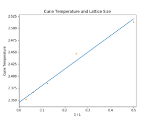Figure 15a: Finding the Curie temperature for an infinite lattice using Python data.
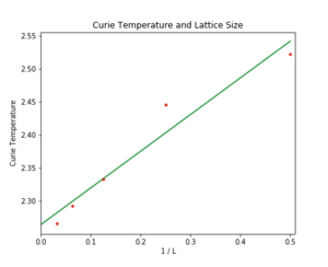Figure 15b: Finding the Curie temperature for an infinite lattice using C++ data.

Conclusion

The Ising model is capable of modelling a variety of physical phenomena in great detail. In this exercise it was used to model ferromagnetic materials by applying the MC Metropolis-Hastings algorithm. Provided large lattice sizes (greater than $16$ ) are sampled for a long time (more than $100000$ iterations), the Curie temperature of an infinite lattice can be found numerically. Any smaller than the mentioned parameters gives numerical inaccuracies which do not reflect well on actual systems. Although first order phase transition can be replicated, what happens at the critical temperature remains a mystery. This problem, along with other curiosities such as non-equilibrium states and higher dimensional Ising lattices, can be featured in further investigations.

Although not explicitly programmed during the exercise, it was demonstrated that for complex N-body systems, lower level languages such as C++ were more rigorous, both in executing more MC iterations in the same amount of time and generating more accurate equilibrium average energy estimates. However data handling, analysis and programming speed was faster for Python.

The Ising model is of course not limited to ferromagnetism. Using the original full Hamiltonian expression in the first section, it is possible to model ionic liquids, colloids or lattice gases ^[8], with the external magnetic field term representing chemical potential (a driving force akin to an external magnetic field for ferromagnetic materials). Applications of the Ising model on other systems or on a system with external driving force can also be featured in further work.

↑ Frenkel and Smit, Understanding Molecular Simulation: From algorithms to applications, Academic Press, 2002
↑ http://farside.ph.utexas.edu/teaching/329/lectures/node110.html#indirect
↑ https://www.britannica.com/science/thermodynamics
↑ https://en.wikipedia.org/wiki/Thermal_fluctuations
↑ Lebon, G., Jou, D., Casas-Vázquez, J. (2008). Understanding Non-equilibrium Thermodynamics: Foundations, Applications, Frontiers, Springer-Verlag, Berlin, e-ISBN 978-3-540-74252-4.
↑ Onsager showed analytically that as the lattice size approaches infinity, the heat capacity converges to a singularity at the Curie temperatureBaxter, Rodney J. (1982), Exactly solved models in statistical mechanics (PDF), London: Academic Press Inc. [Harcourt Brace Jovanovich Publishers], ISBN 978-0-12-083180-7, MR 0690578
↑ K. Binder (2001) [1994], "Ising model", in Hazewinkel, Michiel, Encyclopedia of Mathematics, Springer Science+Business Media B.V. / Kluwer Academic Publishers, ISBN 978-1-55608-010-4
↑ J. Chem. Phys. 149, 164505 (2018); https://doi.org/10.1063/1.5043410

[1] Frenkel and Smit, Understanding Molecular Simulation: From algorithms to applications, Academic Press, 2002

[2] ttp://farside.ph.utexas.edu/teaching/329/lectures/node110.html#indirect

[3] ttps://www.britannica.com/science/thermodynamics

[4] ttps://en.wikipedia.org/wiki/Thermal_fluctuations

[5] Lebon, G., Jou, D., Casas-Vázquez, J. (2008). Understanding Non-equilibrium Thermodynamics: Foundations, Applications, Frontiers, Springer-Verlag, Berlin, e-ISBN 978-3-540-74252-4.

[6] Onsager showed analytically that as the lattice size approaches infinity, the heat capacity converges to a singularity at the Curie temperatureBaxter, Rodney J. (1982), Exactly solved models in statistical mechanics (PDF), London: Academic Press Inc. [Harcourt Brace Jovanovich Publishers], ISBN 978-0-12-083180-7, MR 0690578

[7] K. Binder (2001) [1994], "Ising model", in Hazewinkel, Michiel, Encyclopedia of Mathematics, Springer Science+Business Media B.V. / Kluwer Academic Publishers, ISBN 978-1-55608-010-4

[8] J. Chem. Phys. 149, 164505 (2018); https://doi.org/10.1063/1.5043410

[1]

[2]

[3]

[4]

[5]

[6]

[7]

[8]