Your conclusion isn't that strong and you have a few mistakes in your tasks such as using 1 atom in your fcc unit cell (it's 4) and you lost a 4eps in your LJ algebra but not a bad attempt at the lab. Just remember for your thesis in the future, tailor your intro to an audience and connect your conclusion to your intro (these are your bread and butter). Also have a closer look at heat capacity. Mark: 63/100

Liquid Simulations Computational Lab Assignment - Sam Macer

Abstract

Nicely written, just be careful not to generalise Molecular dynamics simulations of particles interacting according to a Lennard-Jones potential were performed using the velocity-Verlet algorithm. Temperature dependence of density in the NpT ensemble was monitored, and significant deviation from the ideal gas law was observed at low temperatures due to the no collisions assumption breaking down. Heat capacity was monitored as a function of temperature in the NVT ensemble. The radial distribution functions were obtained for solid, liquid and gas systems, as were diffusion coefficients via the mean squared displacement. Furthermore, the diffusion coefficients obtained were realistic; What's a realistic diffusion coefficient? Comparitively reaslistic D (solid) = 1.0 x10⁵m²/s), D (liquid = 3.47 x10⁹m²/s), D (gas = 3.47 x10¹⁰m²/s). Potential industrial applications for such molecular dynamics simulations are also discussed.

Introduction

I like the effort you've put into making your work relevant to a specific audience. The other aspect of a good intro - and I know time was limited - would be to provide a literature review of literature relevant to your audience and your work.

Diffusion is a fundamental form of transport in fluid and soft-condensed phases. All un-equilibrated fluid systems will move via diffusion toward thermodynamic equilibrium This isn't quite true - a system of non-equilibrated particles could very well be ballistic! Think of the msd-t power law! . Many industrial chemical processes could benefit from an optimisation considering diffusion involving the fluid or soft-condensed system being processed. For example, consider piping different coloured icings onto a cupcake to form a pattern. The manufacturer may wish to prevent the diffusion of the two colouring molecules between the bulk of the icing, as this would ruin the pattern. Studying the temperature dependence of this diffusion could allow them to find the maximum temperature at which the cupcake could be safely packaged without significant diffusion occurring.

One study on the extraction of basil essential oil from the Ocimum basilicum leaf exemplifies this¹. The diffusion coefficient was found to change over the course of the extraction; the vapour pressure of the basil oil in the surrounding air increases, while the homogeneity of oil distribution in the leaf diminished as it is depleted from different areas at different rates, due to different tissue structures inside the leaf. The study used models based on Fick’s second law of diffusion, and ultimately elucidated a quadratic relationship between the concentration and diffusion coefficient for the system. This knowledge allows manufacturers to fit the model mathematically using parameters specific to their distillation setup, and use the result to find the best trade-off between extraction time (time and energy are expensive) and extraction yield.

Aims & Objectives

It is absolutely fine, for your thesis, to use bullet points for this section. Makes it neater and to the point!

The aim of this experiment is to use computational models of particles interacting according to a Lennard-Jones potential to extract thermodynamic data about the system and ultimately calculate the diffusion coefficient. The experiment uses boxes of between 1000 and 10000 atoms, with periodic boundary conditions applied to simulate a much larger 'effective system'. The velocity-Verlet algorithm² is used, which iterates the velocity and displacement for every particle in the system, from an initial state, through the desired number of steps. At each of these steps, thermodynamic state variables of the system can be extracted, for e.g. Temperature can be obtained using the average kinetic energies in conjunction with the equipartition theorem.

Reduced units throughout the experiment to make the magnitudes of the quantities used more managable. Given the Lennard-Jones potential:

r = r*/σ

E = E*/ε

T = kT*/ε

r = inter-particle distance, σ = inter-particle distance when the potential = 0, E = potential, ε = depth of the potential well, T = temperature and k = the Boltzmann constant. Starred quantities represent the non-reduced versions. Note the unites cancel out when forming these quantities and hence they are unitless.

By cancelling through these reduced units, we obtain that time is also in reduced units and can be converted via:

Is this an aim/objective?

Methods

This section shouldn't be bullet points - rather an overview of your model followed by the tools/techniques used. It makes it seriously easy to write if you split this into <\model>, <\tool1>, <\tool2> etc.

The open source software, LAMMPS, was used to run the molecular dynamics simulations. The experiment was run as 5 separate parts:

The effect of the time step on the simulation was probed using a box of 1000 atoms, equally spaced with a number density of 0.8 atoms per unit volume. The ensemble was treated as microcanonical. The following time steps were trialed: 0.0150, 0.0100, 0.0075, 0.0025, 0.0010. Energy, temperature and pressure for the system were collected at each iteration. A timestep of 0.0025 was used for the two subsequent simulations - see results and discussion for justification.
A set of simulations (1000 atoms) were run in the isobaric-isothermal (NpT) ensemble. At P = 2.5 & P = 3.0, the simulation was run over the following temperatures: T = 1.5, 2.0, 2.5, 3.5, 5. Density of the systems was extracted as an average after the simulation, and plotted against temperature to test the agreement with the ideal gas law.
An experiment (1000 atoms) was run in the NVT ensemble at densities 0.2 & 0.8, over the temperatures T = 2.0, 2.2, 2.4, 2.6, 2.8. The average heat capacity and temperature were collected for each system.
Simulations (8000 atoms) were performed for a solid, a liquid and a gas system. A timestep of 0.0020 was used. Parameters for this were selected based on a previous probe into the phase transitions of the Lennard-Jones system³; solid (density = 1.2, T = 0.5), liquid (density = 0.8, T = 1.2), gas (density = 0.2, T = 1.2). The output trajectories were used to calculate the RDF (radial distribution function), i.e. the radial frequency of meeting another particle averaged over all spherical angles.
Simulations (8000 atoms) were again performed for a solid, a liquid and a gas phase system. A timestep of 0.0020 was used for this experiment, and the same density/temperature parameters at experiment 4. The MSD (mean squared displacement) was collected as a function of timestep.

Results & Discussion

Experiment 1

These plots show how the thermodynamic state variables of the system vary with time. For all of the variables , we see a very quick convergence from the initial value to the steady state value. A closer inspection of these graphs reveal equilibration happens after roughly 0.5 reduced time units. This shows how the system which is initially ordered quickly descends into chaos. After this point, the state variables proceed to oscillate randomly as a noise function. This occurs due to fluctuations in the system which is constantly moving. If the system had more particles, the average would be less noisy because there are more opportunities for the random imbalances to cancel each other out.

The above plot shows how the energy varies with timestep. As the time step is increased the average energy increases due to the resolution of the numerical solution decreasing. The largest timestep shows a clear divergence. Presumably the timestep is so large that particles are getting unrealistically close to each other. The reaction in the next timestep cascades such that the problem is transferred to neighbouring particles. At this point the simulation breaks down as the energies and particle positions become increasingly unrealistic. 0.0025 was the largest timestep which showed no sign of this increased energy or divergence, and hence the timestep used for all subsequent experiments was smaller than this. Tick

Experiment 2

The density decreases with temperature as expected; the atoms have more kinetic energy, so push each other apart further during their random motion. The higher pressure plots show a consistently higher density. This is intuitive as at higher pressures, the atoms are squashed closer together on average.

At lower temperatures, the ideal gas law result diverges from the simulation. This is because the ideal gas law assumes no collisions. At lower temperatures, particles of an ideal gas continue to be compressed into a smaller space due to their diminishing kinetic energy, such that they are in fact overlapping. In the simulation the particles collide, meaning a much greater kinetic energy (temperature) reduction is required to achieve the same increase in density. Also note that the ideal gas law allows for infinity as the limiting density, whereas this becomes infinitely unlikely when using Van Der Waals potential between the atoms. I don't understand what you mean by infinitely unlikely? Maybe could elaborate more on this point.

Experiment 3

The heat capacity is smaller for lower densities as expected: there are less atoms to sink energy into Maintain your scientific language! , so the average kinetic energy increases more quickly. The heat capacity decreases with temperature because at higher temperatures, the energy states are closer together, meaning it is easier to populate new states (higher density of states). This clearly outweighs any increased degeneracy in states, otherwise we would see the heat capacity increase with temperature as is often the case. The plateau could indicate a first order phase transition where the heat capacity tends to infinity. This would be made more clear with a higher resolution of data points. The radial distribution function could be calculated either side as the less ordered phase would have a smoother curve in the case of a transition. There is a point of confusion here; when you change materials this may be true and it is true that we see a decrease here. But what do you expect for this system? Constant number of particles, constant internal energy (C = dU/dT). Density of states could be a reason for a reduced heat capacity but is it here?

Experiment 4

The radial distribution function (RDF) represents the density of particles around a single particle in the system on average as a function of radius, averaged over all possible angles in a sphere. The RDFs for the different phases are distinct. In the solid case, we se sharp peaks corresponding to when we hit a site in the crystalline lattice. In the liquid, the peaks are much less sharp, as there are many more positions the molecules can occupy easily relative to one another. These peaks are smooth because, in liquid, particles move around more thus you see dynamic averaging. In a solid, we do not see this and the peaks are much more stoccato. The peaks themselves represent long-range order - this is the important point here. Solids have long range order, liquids have less but more than a gas. Peaks are still defined as the distance between particles is roughly constant. A gas behaves like a liquid with very little order. It is less peaks grammar! if any (occur at higher densities) are much less well defined. There is still a sharp peak close to the particle as neighbouring particles spend the most time when changing direction during a collision as this is when velocity is the smallest. All three phases exhibit a cut-off displacement due to the steep positive region in the Lennard-Jones potential.

When the RDF is viewed cumulatively, we see the steepest cumulation for the solid, followed by the liquid then gas. This is due to meeting particles more frequently when walking along the radius in the more dense phase.

Experiment 5

The mean squared displacement plot used the same colours as before to represent a solid, liquid and gas. Initially the MSD is slow to rise, in particular for the gas. This is due to the particles taking some time to disperse properly and reach equilibrium velocity.

The gas has the most freedom and kinetic energy so the MSD is the greatest. The opposite is true for the solid. The liquid is closer to the solid in terms of MSD because it is still relatively ordered, and there is some kind of activation barrier to molecules swapping between cages. The gradient for a solid is effectively zero as swapping positions in a crystalline lattice is extremely rare.

The second plot shows a method of least squared fit, taking into account points after timestep = 1000 only, to avoid data from the equilibration period being considered. The gradients were as following:

Solid: 2.94 x10^-8

Liquid: 1.02 x10^-3

Gas: 1.00 x10^-2

The MSD is related to the diffusion coefficient by a simple relationship:

By simply using this relation, we obtain D as following (in timestep units):

Solid: 4.9 x10^-9

Liquid: 1.7 x10^-4

Gas: 1.7 x10^-3

To convert to the correct units, we must note 1 timestep corresponds to 48.89 fs, therefore we must divide by 49 x10^-15 to get D in SI units:

Solid: 1.0 x10⁵m²/s

Liquid: 3.47 x10⁹m²/s

Gas: 3.47 x10¹⁰m²/s

Which is reasonable as diffusion coefficients for liquids are normally ~ 1 x10⁹m²/s

Now it has been show we can model the diffusion coefficient based purely on molecular dynamics simulations, we can see how similar simulations could be applied to real world applications. In the basil leaf case introduced in the introduction, we could model the leaf structure to follow the real leaf tissue, by using different densities. We would then be able to model accurately how the diffusion of basil essential oil molecules changes as a vapour shell forms and molecules in the leaf are depleted.

Course we could model diffusion coeeficients by MD but the take home message here are the comparisons of your diffusion coefficients and if you'd shown the VACF, comparison between 2 methods to measure the diffusion coefficient.

Conclusion

Not a great conclusion Sam - this should link with your intro and provide a summary for all your key conclusions.

The primary conclusion of this experiment is that molecular dynamics simulations are suitable for physical modelling, and can give more accurate results than ideal solutions such as the ideal gas law. The next step is to begin applying these models to real systems and test their ability to model accurately, such as in the basil leaf case.

The molecular dynamics simulations gave a better estimate of the thermodynamic state variables than the ideal gas law because collisions were included. This is particularly relevant at low temperatures and high pressures. The heat capacity simulations showed that it is possible to observe phase transitions between phases. The RDF is a unique insight that would be much more difficult to measure in reality. It is a useful tool as is gives us detailed information on the structure of the system being studied. In a solid for example, the RDF peaks can be correlated to crystalline lattice sites. Having access to the displacements and velocities of each particle allows us to calculate a wealth of parameters, the diffusion coefficient being just one example. Obtaining a realistic diffusion coefficient implies that the method models the system realistically.

It is clear that the amount of important data that can be quickly obtained for a system simulated using molecular dynamics is immense. is immense scientific? It would be recommended that such methods are tested against real world experiments to gain a better understanding of their accuracy.

References

J. Silveira, A. Costa and E. Costa Junior, Engenharia Agrícola, 2017, 37, 717-726.
L. Verlet, Physical Review, 1967, 159, 98-103.
J. Hansen and L. Verlet, Physical Review, 1969, 184, 151-161.

Weblinks:

http://www.scielo.br/scielo.php?script=sci_arttext&pid=S0100-69162017000400717#B21
https://journals.aps.org/pr/abstract/10.1103/PhysRev.159.98
https://journals.aps.org/pr/abstract/10.1103/PhysRev.184.151

Appendix

Previously unanswered tasks: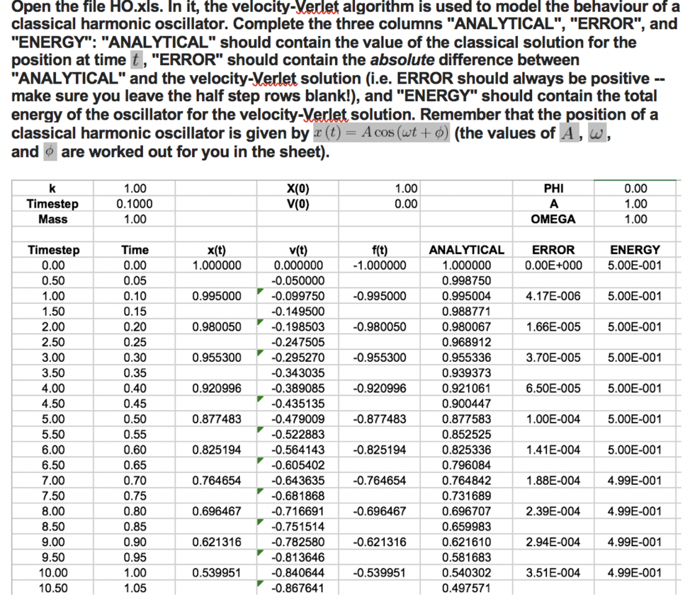

Your algebra in calculation of equiblirium distance and well depth isn't right - you've lost a 4eps

Does an fcc unit cell contain only 1 atom? dens = N/l^3. fcc unit celll contains 4 atoms!

LAMMPS script for heat capacity experiments:

### DEFINE SIMULATION BOX GEOMETRY ###

variable dens equal 0.2

lattice sc ${dens}

region box block 0 15 0 15 0 15

create_box 1 box

create_atoms 1 box

### DEFINE PHYSICAL PROPERTIES OF ATOMS ###

mass 1 1.0

pair_style lj/cut/opt 3.0

pair_coeff 1 1 1.0 1.0

neighbor 2.0 bin

### SPECIFY THE REQUIRED THERMODYNAMIC STATE ###

variable T equal 2.0

variable timestep equal 0.0075

### ASSIGN ATOMIC VELOCITIES ###

velocity all create ${T} 12345 dist gaussian rot yes mom yes

### SPECIFY ENSEMBLE ###

timestep ${timestep}

fix nve all nve

### THERMODYNAMIC OUTPUT CONTROL ###

thermo_style custom time etotal temp press

thermo 10

### RECORD TRAJECTORY ###

dump traj all custom 1000 output-1 id x y z

### SPECIFY TIMESTEP ###

### RUN SIMULATION TO MELT CRYSTAL ###

run 10000

unfix nve

reset_timestep 0

### BRING SYSTEM TO REQUIRED STATE ###

variable tdamp equal ${timestep}*100

fix nvt all nvt temp ${T} ${T} ${tdamp}

run 10000

reset_timestep 0

unfix nvt

fix nve all nve

### MEASURE SYSTEM STATE ###

thermo_style custom etotal temp atoms vol

variable vol equal vol

variable atoms equal atoms

variable temp equal temp

variable temp2 equal temp*temp

variable N2 equal atoms*atoms

variable E2 equal etotal*etotal

variable E equal etotal

fix aves all ave/time 100 1000 100000 v_temp2 v_E v_E2

run 100000

variable heatcapac equal ${N2}*(f_aves[3]-(f_aves[2]*f_aves[2]))/(f_aves[1])

print "Averages"

print "--------"

print "Heat Capacity: ${heatcapac}"

print "Volume: ${vol}"

print "No of atoms: ${atoms}"