Rep:Nm1916cmp
Simulation of 2D Ising Model Using the Monte Carlo Method
Introduction
An experiment into modelling a 2D Ising Lattice using object orientated programming (OOP) and the Metropolis Monte Carlo (MMC) simulation was conducted to investigate the effect of lattice size and temperature on the 2D Ising lattice. Thermodynamic properties of the system were then studied including heat capacity and the Curie temperature. Finally, the thermodynamic properties were compared to those of another simulation that was run on a different programming language.
Any code and simulation used was created with Python 3.6.3 run in Spyder 3.1.4 environment unless mentioned otherwise. [1]
The Ising Model
The Ising model is a statistical mechanics model used to describe the behaviour of ferromagnetic materials. In ferromagnetic materials the magnetic dipole moment of the atoms is either +1 or -1, corresponding to whether the spins point up or down. There are certain constraints within the model:
- In the absence of external magnetic fields, the only interactions which contribute to the energy of the system come from spins in cells adjacent to each other.
- The interaction energy E is defined as where J is a constant relating to the strength of interactions between adjacent lattice cells.
- Periodic boundary conditions are applied - the lattice is infinitely repeating.
Task 1- Show that the lowest possible energy for the Ising model is E = -DNJ, where D is the number of dimensions and N is the total number of spins. What is the multiplicity of this state? Calculate its entropy.
From above,
If D is the number of dimensions you consider then there are 2D interactions for each dipole as only interaction with neighbouring spins are included within the model. For example, in 2D space a magnetic dipole will interact with 4 other dipoles. The lowest possible energy of the system is one in which all the spins are parallel in either direction. In this case
Therefore:
Summing over the number of particles N each with 2D interactions gives:
The factor of is included to prevent interactions being double counted.
There are 2 degenerate lowest energy states, when the spins are all parallel aligned up or down. These states are not in equilibrium, however they are indistinguishable in the absence of external magnetic fields. Therefore the number of ways the system can align at the lowest energy state is 2.
From:
The entropy of the lowest energy state in the Ising model is:
Phase Transitions
TASK 2: Imagine that the system is in the lowest energy configuration. To move to a different state, one of the spins must spontaneously change direction ("flip"). What is the change in energy if this happens (D=3, N=1000)? How much entropy does the system gain by doing so?
In 3D space each magnetic dipole has 6 neighbours in which it interacts with. If all the dipoles were aligned parallel either pointing up or pointing down, using the energy of the system would be .
If one of the magnetic dipoles flipped directions, 6 favourable interactions between parallel spins would be lost, whilst 6 unfavourable interactions between dipoles of opposite spin would also occur. Therefore the energy of the system would be raised by 12J and would be .
The entropy of the new state can be calculated from .
for the new energy state is going to be which is 2000. The factor of 2 comes from the fact that the system could align with 999 upwards spin and 1 downwards spin or vice versa. Therefore the entropy of the new state is:
The entropy of the original state is :
Therefore, the change in entropy is:
TASK 3: Calculate the magnetisation of the 1D and 2D lattices in figure 1. What magnetisation would you expect to observe for an Ising lattice with at absolute zero?
For both the 1D and 2D lattice, the magnetisation is .
For a lattice with the magnetisation will either be or depending on which direction the spins point. This comes from the 3rd law of thermodynamics which states that the entropy at 0 K has to be 0 therefore which corresponds to all the spins aligning in the same direction.
Calculating the Energy and Magnetisation
TASK 4 : complete the functions energy() and magnetisation(), which should return the energy of the lattice and the total magnetisation, respectively. In the energy() function you may assume that at all times (in fact, we are working in reduced units in which , but there will be more information about this in later sections). Do not worry about the efficiency of the code at the moment — we will address the speed in a later part of the experiment.


Figure 1 and 2 show the original functions used to calculate the energy and magnetisation for the Ising Lattice. The energy is calculated in the same way as described above, by only considering interactions with neighbouring spins. Since the system considered is in 2D, each lattice point will have 4 neighbours hence the 4 different variables defined above, as well as the central lattice that is being considered. However, this could have been more efficient as only 2 interactions instead of 4 need to be considered. By only considering interactions with spins above and spins to the right, the factor of 1/2 in the energy function could be removed, and 2 less variables would need to be defined. However the energy function was improved again later so this did not have a big impact on run time.
The energy function is originally set to be 0. It then it takes into account the interaction of each spin with its surrounding neighbours and then calculates the total energy. The size of the lattice is controlled by n_rows and n_columns which are parameters of the __init__ method within the class IsingLattice as seen in Figure 3.
The modulo function % allows for an infinite lattice and periodic boundary conditions. E.g. for a 3x3 lattice, column 3 on one lattice neighbours with column 1 on the lattice beside it and the modulo function allows for these to interact.
The magnetisation function in figure 3 sums up all the spins within the lattice and returns the value of the total magnetisation of the lattice. The magnetisation function was not changed throughout the experiment.
** The screenshots above were taken a while ago and the code has been changed since, hence the code was not annotated. All further code within this experiment will be annotated.**
TASK 5: Run the ILcheck.py script from the IPython Qt console using the command %run ILcheck.py and show the figure.

ILcheck.py is a script which generates 3 4x4 lattices, one which should give the lowest energy state, one which gives the highest energy state and one which is in between. It then generates an image that represents this and gives values for the total energy and total magnetisation for each state. The images in Figure 4 shows that both the energy and magnetisation functions from Figure 1 and Figure 2 are correct and represent the infinite lattice. The first image in Figure 4 corresponds to the lowest energy state in which all the spins are parallel with the highest magnetisation and the last image corresponds to the highest energy state when all the spins are antiparallel and the magnetisation is 0.
Introduction to the Monte Carlo Simulation
TASK 6: How many configurations are available to a system with 100 spins? To evaluate these expressions, we have to calculate the energy and magnetisation for each of these configurations, then perform the sum. Let's be very, very, generous, and say that we can analyse configurations per second with our computer. How long will it take to evaluate a single value of ?
If the system has 100 spins which can take 2 values, +1 or -1, then the number of possible configurations Ω is given by 2100.
The time taken to evaluate the magnetisation will be:
seconds which is years.
TASK 7: Implement a single cycle of the above algorithm in the montecarlocycle(T) function. This function should return the energy of your lattice and the magnetisation at the end of the cycle. You may assume that the energy returned by your energy() function is in units of ! Complete the statistics() function. This should return the following quantities whenever it is called: , and the number of Monte Carlo steps that have elapsed.
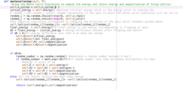

The Metropolis Monte Carlo(MMC) is an algorithm which works by random sampling, in this case, to lower the energy of the system.
The steps are described by the comment on the code. A random lattice is selected and the spin flipped. If the flipped spin is of lower energy than the original spin, the new configuration is accepted. If not a random number between 0 and 1 is generated. If the random number generated is less than the Boltzmann distribution using the difference between the final and initial energy, the new configuration is kept. If not, the configuration is rejected and the configuration is returned to the original configuration.
The code could have been more efficient as could have set the rejected configuration as an if statement and then used an else statement for both other configurations. This is improved later in the experiment.
TASK 8: If , do you expect a spontaneous magnetisation (i.e. do you expect )? When the state of the simulation appears to stop changing (when you have reached an equilibrium state), use the controls to export the output to PNG and attach this to your report. You should also include the output from your statistics() function.
Below the Curie temperature spontaneous magnetisation is expected. The system aligns in a way to minimise the free energy of the system. This is a balance between the internal energy U and the entropy S of the system.
The Helmholtz Free Energy is defined as:
At low temperature the entropy of the system has little impact on the free energy, therefore the system will often align with all the spins parallel in order to minimise the internal energy as was shown in Task 1. As temperature increases the entropic component has more of an impact on the free energy and at a certain point, Tc , ferromagnetic materials become paramagnetic - the spins are randomly orientated (in the absence of an external magnetic field). Here the repulsion between non parallel spins and the loss of favourable interactions between parallel spins is outweighed by the huge increase in entropy.
The file ILanin.py was run at 1 K to investigate what happened to the energy and magnetisation of the Ising Lattice over time.*
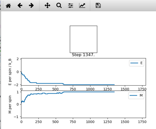

The file generates an 8x8 lattice and measures the energy and magnetisation per spin as the number of steps increases. The temperature this is run at is below Tc therefore the trend observed is expected. The energy of the system decreases and the magnetisation tends towards and then equals a value of +1 or -1 as the number of steps increases. This corresponds to more parallel spin alignments increasing with time which results in the decrease in energy. The magnetisation tends towards 1 for the reasons described above as we are below Tc . The magnetisation could have equally tended towards and then towards -1 which would correspond to the spins still having a parallel arrangement but pointing in the opposite direction. Whether it tends towards +1 or -1 is largely dependant on initial random spin states generated.
It is possible for the magnetisation and energy not to reach a global minimum, it can get stuck in a local minimum. In this case, the magnetisation will not tend towards 1 or -1 and the energy would not be the minimum possible energy for the system. To get to the global minimum from this local potential well, usually an increase in temperature, collisions or thermal fluctuations can cause this to occur in real systems.
The values generated for the energy and magnetisation do not make much sense. We would expect the energy per spin to be very close to -2 J and the average magnetisation to be close to +1 or -1. This is not what is seen in Figure 8. The reason for this is the calculation of both the average energy and average magnetisation include the values up to 600 steps which is before equilibrium was reached. This means that for almost half the simulation(1363 steps) the system was not in equilibrium which explains why the expected results were not achieved. This is improved later in the experiment with only energy and magnetisation values after equilibrium included in the average values.
*ILanim.py simulation would not run in the iPython console within Spyder therefore was ran in terminal.
Accelerating the Code
TASK 9: Use the script ILtimetrial.py to record how long your current version of IsingLattice.py takes to perform 2000 Monte Carlo steps. This will vary, depending on what else the computer happens to be doing, so perform repeats and report the error in your average!
The average time taken to run 2000 Monte Carlo steps using the energy function in Task 4 was 32.9516 seconds which is very long. This may partly be due to calculating all 4 interactions for each spin instead of just 2.
TASK 10: Look at the documentation for the NumPy sum function. You should be able to modify your magnetisation() function so that it uses this to evaluate M. The energy is a little trickier. Familiarise yourself with the NumPy roll and multiply functions, and use these to replace your energy double loop (you will need to call roll and multiply twice!).

The double loop in calculating the energy took a long time to run as shown above, therefore was replaced with a numpy function numpy.roll (numpy was imported as np at beginning of script).
The roll function works by taking an array and translating it in a direction along an axis. As described in Task 4 only one interaction along the x axis and one along the y axis needs to be calculated to take into account all the interactions of spin. The lattice is translated along an axis and then multiplied by the original lattice. The interactions are then summed together to give a total energy value.
TASK 11: Use the script ILtimetrial.py to record how long your new version of IsingLattice.py takes to perform 2000 Monte Carlo steps. This will vary, depending on what else the computer happens to be doing, so perform repeats and report the error in your average!
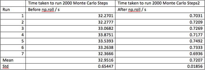
Figure 8 shows the average time taken to run 2000 Monte Carlo steps before and after using np.roll . The new energy function is over 45 times quicker than the previous one. This is important as later in the experiment there would be 100000 Monte Carlo steps being run.
The standard deviation before and after the roll function barley changed (1.99% and 2.57% respectively). The fluctuations arise from other programmes on the computer using processing power and this changes over time. The fluctuations are very small and have no significant impact on running the simulation.
The Effect of Temperature
TASK 12: The script ILfinalframe.py runs for a given number of cycles at a given temperature, then plots a depiction of the final lattice state as well as graphs of the energy and magnetisation as a function of cycle number. This is much quicker than animating every frame! Experiment with different temperature and lattice sizes. How many cycles are typically needed for the system to go from its random starting position to the equilibrium state? Modify your statistics() and montecarlostep() functions so that the first N cycles of the simulation are ignored when calculating the averages. You should state in your report what period you chose to ignore, and include graphs from ILfinalframe.py to illustrate your motivation in choosing this figure.
ILfinalframe.py shows the final lattice as well as the energy and magnetisation per spin for the number of steps run (100000). At temperatures below Tc the system usually adopts the lowest energy state in order to decrease the free energy of the system, although sometimes the system may get stuck in a metastable state in which the internal energy of the system is not minimised.
It is clear that at the size of a lattice has a big effect on the time taken for the system to reach equilibrium, larger lattices take much longer.
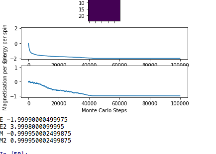

For an 8x8 lattice at 1K it takes somewhere between 1000-2000 steps for equilibrium to be reached. Whereas for a 25x25 lattice at 1K it takes somewhere between 40000 and 50000 steps for equilibrium to be reached. This is because the Monte Carlo step is going to have to go through a lot more lattice points within the larger system in order to lower the total energy of the system. Larger systems are also more likely to be found in a metastable state, one non parallel spin has much less of an effect in a larger system.
The energy and magnetisation values are what we expect for a lattice at equilbrium. The modifications to the Monte Carlo method and statistics function are shown further down.
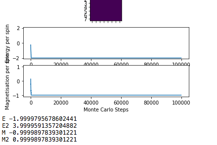


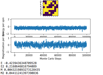
Temperature also has a large impact in the time taken to reach equilibrium. At lower temperatures equilbrium tends to be reached quicker. It is clear there is not much difference in time taken to to reach equilibrium between 0.1 K and 1 K however 1K does reach equilbrium quicker. Both of these temperatures are below the Curie Temperature. Equilbrium is not reached for the 8x8 lattice at 1.5 K. This temperature is approaching Tc and the system did not equilibrate fully, it fluctuated around the minimum energy. The system did still try to minimise energy.
After Tc equilibrium is reached at 0 cycles. The Ising Lattice is in random equilbrium after Tc which results in large fluctuations in both the magnetisation and energy per with number of cycles. The entropic component of the free energy is dominant therefore the system does not attempt to minimise the internal energy by aligning parallel spins and instead the system becomes disordered. The graph for 3 K looks the same as at 5 K and 7K.
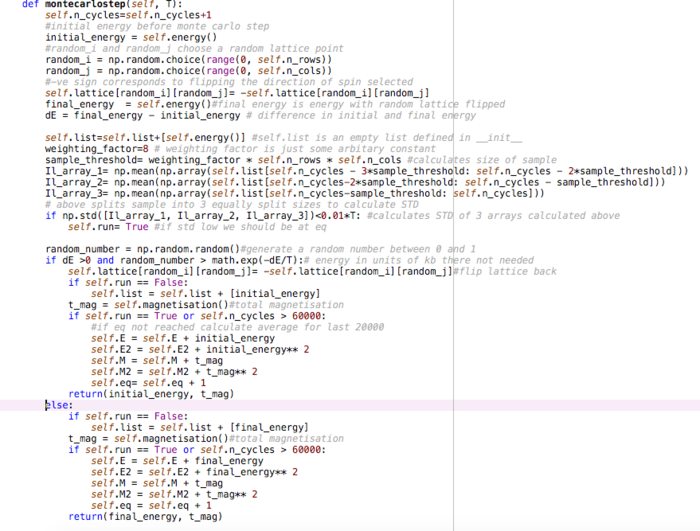
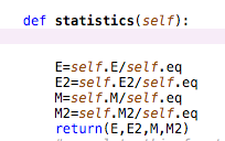
The Monte Carlo and Statistics function have been updated in order to calculate the average energy and magnetisation after equilibrium has been reached. The approach taken was to automate the code to find the equilibrium point for you. This was done by finding the standard deviation of 3 different sections of the graph and if it was very low then we would say the system was at equilibrium. However, there was a clause that found the average after 60000 steps if equilibrium had not been reached. This was generally quite a successful method however it increased the run time of the code significantly. Statistics were divided by the number of cycles after equilbrium now instead of n_cycles.
TASK 13: Use ILtemperaturerange.py to plot the average energy and magnetisation for each temperature, with error bars, for an lattice. Use your intuition and results from the script ILfinalframe.py to estimate how many cycles each simulation should be. The temperature range 0.25 to 5.0 is sufficient. Use as many temperature points as you feel necessary to illustrate the trend, but do not use a temperature spacing larger than 0.5. The NumPy function savetxt() stores your array of output data on disk — you will need it later. Save the file as 8x8.dat so that you know which lattice size it came from.
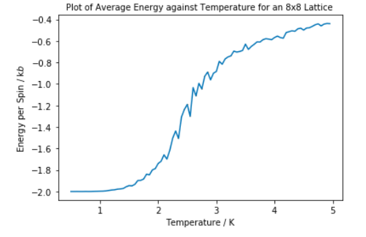
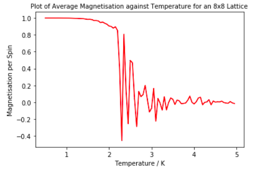
ILtemperaturerange.py was used to show how the average energy and magnetisation per spin of an Ising Lattice varied as temperature increases. The temperature was measured between 0.5 and 5 K in steps of 0.05 K with 80000 steps being run at each temperature.
There are error bars of standard error on both Figure 11 and Figure 12 but they are not visible showing how low the error in the calculation is.
The average energy increases as the temperature increases. This is due to the entropic component of the free energy having more of a contribution as temperature increases. After Tc the entropic component significantly outweighs the internal energy contribution and there is a random thermal equilibrium set up between the magnetic spins. At very low temperatures the energy per spin tends towards -2 J. This comes from Task 1:
Since the model is for a 2D Ising Lattice, D=2. The energy is measured per spin therefore is independent of N. This would correspond to all the spins being aligned parallel. There is significantly more fluctuation in the middle region of the energy per spin against temperature graph. Somewhere within this region lies Tc which is the reason for the fluctuations. As temperature increases towards the Tc the balance of internal energy and entropy balances out which is seen as fluctuations.
The magnetisation per spin starts at a value of +1, as at lower temperature it is more favourable for the system to have all the spins aligned parallel as entropic component has very little contribution to the free energy. The magnetisation slowly decreases until near Tc there is a sharp decrease in the magnetisation. It however seems the drop in magnetisation, especially in smaller system, is before Tc. At this point it is more favourable for the system to be more disordered, hence the the spins are no longer arranged parallel. After this the magnetisation per spin fluctuates around 0 as the spins are randomly aligned.
The Effect of System Size
TASK 14: Repeat the final task of the previous section for the following lattice sizes: 2x2, 4x4, 8x8, 16x16, 32x32. Make sure that you name each datafile that your produce after the corresponding lattice size! Write a Python script to make a plot showing the energy per spin versus temperature for each of your lattice sizes. Hint: the NumPy loadtxt function is the reverse of the savetxt function, and can be used to read your previously saved files into the script. Repeat this for the magnetisation. As before, use the plot controls to save your a PNG image of your plot and attach this to the report. How big a lattice do you think is big enough to capture the long range fluctuations?
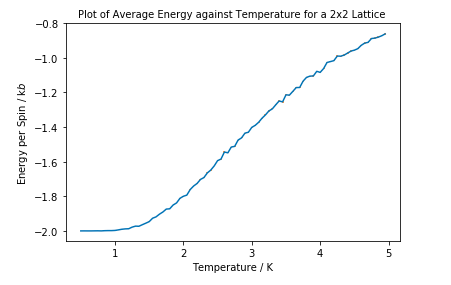
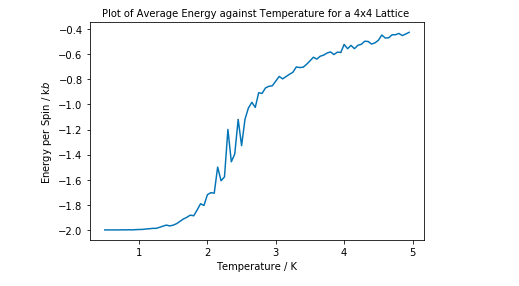

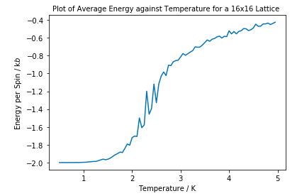

ILtemperaturerange.py was run for the same settings as Task 13. The simulation, especially for 16x16 and 32x32 lattice sizes took quite a long time to run. There are error bars of standard error plotted on all graphs but the error is very low therefore not observable.
For reasons discussed above, the energy starts at -2J. It then increases as temperature increases as the entropic component contributes more. The larger the lattice size, the steeper the region around Tc. This indicates there is less of a region in which there is a balance between internal energy and entropy, and that entropic component has a larger effect on the overall free energy of the system earlier.
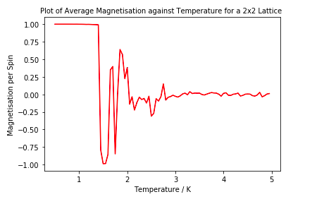
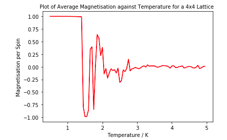


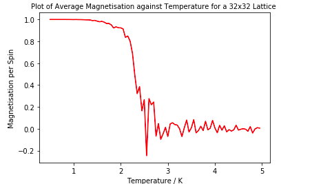
It is clear that as the Ising Lattice increases in size, that the magnetisation per spin falls at a higher temperature. In a smaller system it is easier to change the spins from being parallel to being random as Tc is approached as much less spins need to change orientation for this to occur.
The magnetisation per spin follows the same trend for all lattice sizes. It starts at +1 at low temperature due to the all spins being parallel as internal energy is the major contribution to the free energy. The magnetisation slowly decreases until near Tc where there is a sharp decline in the magnetisation per spin due to the entropic disorder factor having a larger contribution to the free energy, therefore it fluctuates around 0.
In a smaller system the magnetisation falls much before Tc possibly due to a shallow energy profile for the smaller systems.
Heat Capacity
TASK 15: By definition,
From this, show that
(Where is the variance in .)
From statistical thermodynamics we know that:
The variance of U is the rate of change of U with thermal fluctuations. Therefore:
By definition the heat capacity C:
Using the product rule:
Since:
And
TASK 16: Write a Python script to make a plot showing the heat capacity versus temperature for each of your lattice sizes from the previous section. You may need to do some research to recall the connection between the variance of a variable, , the mean of its square , and its squared mean . You may find that the data around the peak is very noisy — this is normal, and is a result of being in the critical region. As before, use the plot controls to save your a PNG image of your plot and attach this to the report.

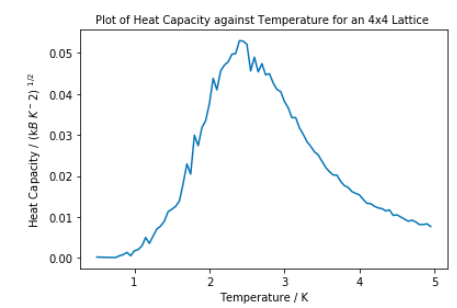
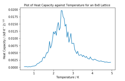
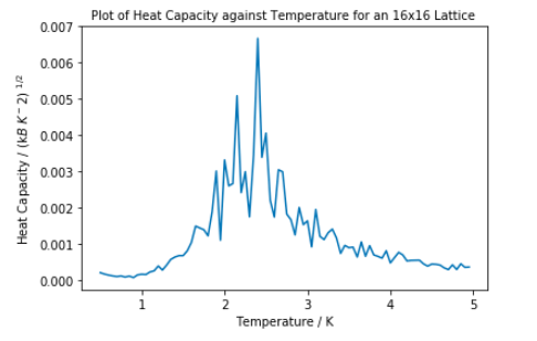
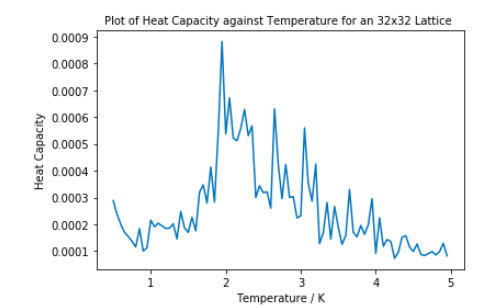
The heat capacity was calculated using the derivation above. The same temperature spacing and number of steps was used as in Task 13 and Task 14.
From the 2D Ising model, it would be expected that heat capacity would diverge towards infinity at Tc as it is a phase transition. [2] This does not happen in any of the lattices above. However the maximum peak within the critical region does increase in sharpness as lattice size increases. In further investigations into this area, the lattice size should be increased to 64x64 and 128x128 to investigate whether the larger system will cause divergence of the heat capacity at Tc.
The reason for the increased fluctuations for bigger lattice sizes as temperature increases may be due to the balance between the entropic and internal energy of the system. As temperature increases, the internal energy has less of an impact on the system which would result in the energy of the system fluctuating more as the orientation of parallel spins has less of an impact. Since in a larger lattice, one spin changing would effect the energy of the system less than in a smaller system, more energy therefore heat capacity fluctuations are seen.
The heat capacity plotted is heat capacity per spin squared. It has the same shape as heat capacity per spin, just lower values. Either one can be used to find the Curie Temperature as it is at maximum temperature, not heat capacity.
Locating the Curie Temperature
TASK 17: A C++ program has been used to run some much longer simulations than would be possible on the college computers in Python. You can view its source code here if you are interested. Each file contains six columns: (the final five quantities are per spin), and you can read them with the NumPy loadtxt function as before. For each lattice size, plot the C++ data against your data. For one lattice size, save a PNG of this comparison and add it to your report — add a legend to the graph to label which is which. To do this, you will need to pass the label="..." keyword to the plot function, then call the legend() function of the axis object (documentation here).
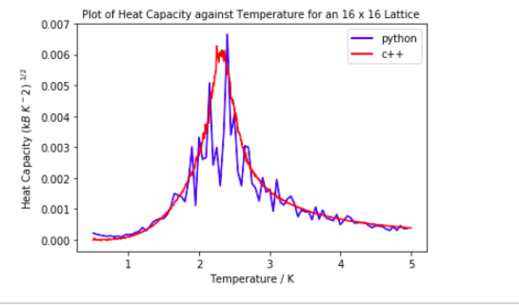
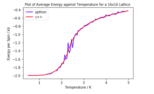
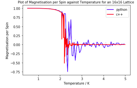
Above shows the Python data plotted along with C++ data for a 16x16 lattice. It is clear the data is very similar and overlaps quite well.
The energy per spin data maps onto each other very well with the C++ plot having less noise in the critical region. This is possibly due to the C++ data being collected from a simulation which was run for much longer. However the general shape and values match up very well.
The heat capacity from the python data map onto the C++ data very well, however the maximum value for the python data is shifted to a slightly higher temperature. This is due to the python data being very noisy within the critical region. We would however expect the peak to diverge at Tc which it seems to do more so in python than C++. However, we have a finite system of small size therefore the peaks are more rounded. As lattice size increases, the peak would be expected to increase in size and diverge more.
The magnetisation per spin from the python maps onto the C++ data quite well. However, the point in which the magnetisation has a sharp decrease around Tc is slightly earlier. The C++ data also only has very small fluctuations around 0 and higher temperatures whereas the python data still fluctuates a lot more.
Smaller lattice sizes map the python onto the C++ better than the 16x16 and 32x32.
TASK 18: write a script to read the data from a particular file, and plot C vs T, as well as a fitted polynomial. Try changing the degree of the polynomial to improve the fit — in general, it might be difficult to get a good fit! Attach a PNG of an example fit to your report.

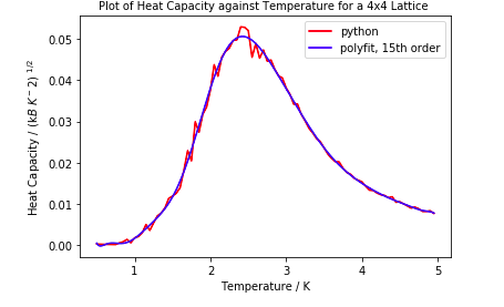
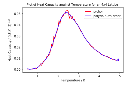
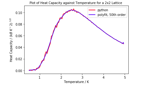

Above is graphs of the heat capacity of different size lattices against temperature and a fitted graph using np.polyfit and np.polyval. It is clear that quite a high order polynomial is required to fit the data. The higher order, the more terms used to in the fitting therefore a more accurate curve is generated. It is clear that for a 4x4 lattice, the polynomial fit is the order of 5 as the it does not map very well. Through trial and error it was found that the order to fit for a 4x4 lattice is around 15. Increasing the order above this did not fit the graph any better.
Lattice sizes of higher order require higher order polynomials to fit. From above it is evident that an order of 50 for the 8x8 lattice fits well generally but not at the peak whereas a 50 order polynomial mapped onto 2x2 data almost perfectly. This is because as lattice size increases, the peak in the heat capacity vs temperature graph which represents the phase transition is more likely to diverge, therefore it is harder to fit a curve to it.
TASK 19: Modify your script from the previous section. You should still plot the whole temperature range, but fit the polynomial only to the peak of the heat capacity! You should find it easier to get a good fit when restricted to this region.
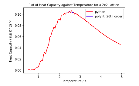
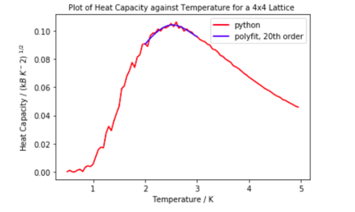
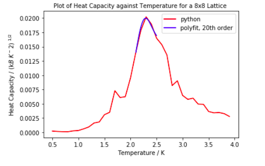
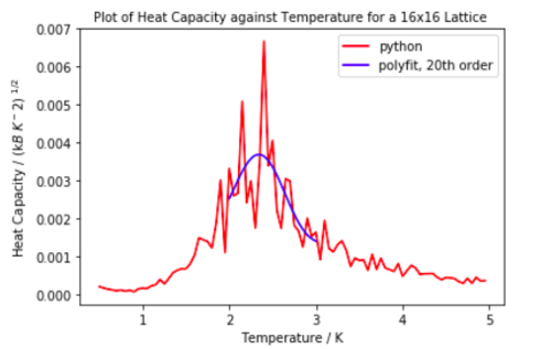
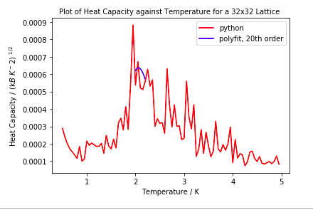

All graphs above were fitted with polyfit using an order of 20. Above this there did not seem to be any noticeable improvement in fitting to the peak.
Above is the heat capacity against temperature plot for all lattice sizes as well as polyfitted curves and a table showing the maximum temperature value. Tc decreases with increasing lattice size, possibly due to long range fluctuations. Tc for the 32x32 lattice is lower than literature value for the infinite lattice<quote>. This is because as the lattice size increases, the more the graph starts to diverge, therefore it is very difficult to fit a polynomial graph onto it. The large fluctuations within the critical region also make it difficult to distinguish which is the peak which corresponds to the phase transition.
The polyfit curves fit very nicely onto smaller lattice sizes which is probably a result of the finite size effect.
Although for the larger lattices, the curve does not map onto the correct heat capacity values, it is only the maximum temperature that is being considered, therefore as long as the peak is correct on the x-axis it is acceptable.
Limiting the range of where the polyfit was calculated improved the fit considerably.
TASK 20: find the temperature at which the maximum in C occurs for each datafile that you were given. Make a text file containing two colums: the lattice side length (2,4,8, etc.), and the temperature at which C is a maximum. This is your estimate of for that side length. Make a plot that uses the scaling relation given above to determine . By doing a little research online, you should be able to find the theoretical exact Curie temperature for the infinite 2D Ising lattice. How does your value compare to this? Are you surprised by how good/bad the agreement is? Attach a PNG of this final graph to your report, and discuss briefly what you think the major sources of error are in your estimate.

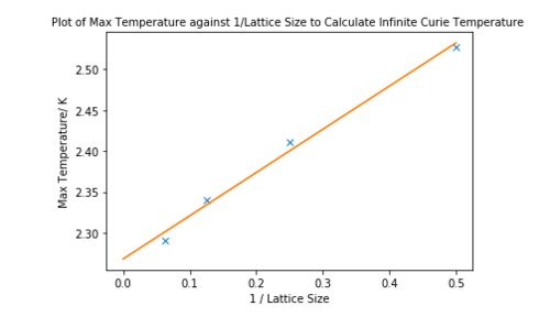
The maximum temperature against 1 / lattice size was plotted in an attempted to find .
From:
The Y intercept was equal to where A is an constant and L is length of one the sides of the lattice.
As discussed above, the Tc for the 32x32 lattice was not able to be calculated accurately. When finding using all lattice points, it was found to be 2.1815 K which is lower than calculated in literature. The reason for this was due to difficulty in fitting polyfit to the large sharp peaks. This point was therefore ignored.
When ignoring Tmax for the 32x32 lattice, was found to be 2.2680 K which is extremely close to literature value of 2.2691 K. [3]It is correct to 2 d.p. which is extremely close considering the error associated with curve fit. This was found only using 4 data points however, therefore in the future many more square lattices should be used to give this calculation more validity. It is surprising how close to literature value was obtained, even when considering the 32 x 32 lattice which is only around 4% different.
The main sources of error in the calculation was using polyfit in an attempt to model a curve which, in theory, should diverge. Also, the accuracy was limited by the run time and number of steps that were able to be run on python. As seen when using C++ data, which was a much larger simulation, the graphs obtained were much smoother and fluctuated much less.
Conclusion
The simulation successfully modelled a 2D Ising lattice obtaining a value of within 2 d.p to literature values. For relatively simple code and simulations run it was quite accurate. It is a good investigation to introduce object orientated programming and simple computer algorithms (MMC) whilst also being able to interpret and relate the findings to physical chemistry phenomena. In future experiments, the simulation run should be much larger and for much larger size lattices in an attempt to get the heat capacity to diverge without much noise in the critical region as seen in the C++ data. This would allow the Tc to be found without using curve fitting, which introduced large source of error into the experiment.
References
- ↑ Fernando Bresme, Ollie Robotham, "Third year CMP compulsory experiment/Introduction to Monte Carlo simulation", https://wiki.ch.ic.ac.uk/wiki/index.php?title=Third_year_CMP_compulsory_experiment/Introduction_to_Monte_Carlo_simulation
- ↑ John Orehotsky* and Klaus SehrSder, "Specific Heat of Nickel-Iron and Nickel-Cobalt Alloys between 600 ~K and 1500 ~K ", Phys Cond Matter, 1973, 17, 37-53.
- ↑ https://en.wikipedia.org/wiki/Square-lattice_Ising_model
