Rep:NasCOMP

Nas' CMP Comp

The purpose of this exercise was to model a low temperature 2D lattice of a para-magnetic solid. In particular the cross-over point of the enthalpic and entropic regimes was studied using a Monte Carlo simulation. Please note that all temperatures and energies stated in this exercise are in reduced units of Kb. Heat capacity is therefore in units of Kb^-1.

Ising Model

The interaction energy is defined as $$\begin{gathered} -\frac{1}{2}J\sum _i^N\sum _{j \\ \in \\ \mathrm{n}\mathrm{e}\mathrm{i}\mathrm{g}\mathrm{h}\mathrm{b}\mathrm{o}\mathrm{u}\mathrm{r}\mathrm{s}\left(i\right)}{s}_i{s}_j \end{gathered}$$, where $J$ is a constant which controls the strength of interaction and the notation $$\begin{gathered} j \\ \in \\ \mathrm{n}\mathrm{e}\mathrm{i}\mathrm{g}\mathrm{h}\mathrm{b}\mathrm{o}\mathrm{u}\mathrm{r}\mathrm{s}\left(i\right) \end{gathered}$$ indicates that spin $j$ must lie in a lattice cell adjacent to spin $i$.

TASK: Show that the lowest possible energy for the Ising model is $$\begin{gathered} E \\ = \\ -DNJ \end{gathered}$$, where $D$ is the number of dimensions and $N$ is the total number of spins. What is the multiplicity of this state? Calculate its entropy.

By viewing the above equation we realise that in order to miminise the energy of the system we must maximise the total sum of spin-spin interactions. This occurs when all spins are aligned. In a 1D system of N atoms, each atom has 2 interactions: one with the atom each side). We also can apply periodic boundary conditions so an end atom interacts with first atom in the chain. However we need to now recognise that spin ₁*spin₂ is the same as spin₂*spin₁ and as such we need to halve the total number of spin terms that appear in the sum.

=> E = -0.5*J*N*2 =>  E = -DJN

We can make analogous arguments for 2D and 3D lattices, where each atom interacts with 4 and 6 neighbors respectively:

2D: E= -0.5*J*N*4 
3D: E=-0.5*J*N*6   

both also yield the general equation:

E=-DJN.

This result has some theoretical basis since we know from Hund's Rule of Maximum Multiplicity that fermions in degenerate energy levels adopt parallel spins in order to minimise their total energy. This occurs since parallel spins miminise the shielding of nuclear charge (electric field) experience by the other electrons in the atom.

The multiplicity of this energy level is 2 as spins can be all parallel up or all parallel down. Entropy will be S= K_Bln2 .

TASK: Imagine that the system is in the lowest energy configuration. To move to a different state, one of the spins must spontaneously change direction ("flip"). What is the change in energy if this happens ($$\begin{gathered} D=3, \\ N=1000 \end{gathered}$$)? How much entropy does the system gain by doing so?

Flipping one spin in a 3D lattice changes 6 stabilising interactions into destabilising interactions. Not only does this mean there is an increase in the energy of the system from the removal of the 6 stabilising interactions, but the destabilsation further cancels out 6 more stabilising alignments. From this logic we can make a simple modification to our equation for total energy: E=-DNJ => -DJ(N-4n) - where n is the number of anti-aligned spins isolated in the parallel spin lattice. The energy of the second lowest energy state in the system states is therefore 12J higher than the lowest state. The degeneracy is 2*1000, as every atom could be spin up whilst the others are spin down and visa versa. Change in Entropy ΔS= k_bln (2000/2)

TASK: Calculate the magnetisation of the 1D and 2D lattices in figure 1. What magnetisation would you expect to observe for an Ising lattice with $$\begin{gathered} D=3, \\ N=1000 \end{gathered}$$ at absolute zero?

Magnitisation is simply the sum of all spins. For the lattices shown in Fig1.

1D: Total Magnetisation = 3*(1)+2*(-1)=1 2D: Total Magnetisation = 13*(1)+12*(-1)=1

For a 3D lattice at 0°K we would expect all spins to be parallel therefore M = 1000

Magnetisation and Energy Calculations with Python

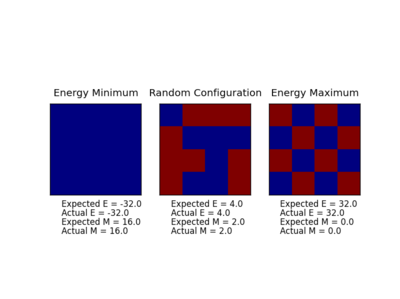
The IsingLattic.py was completed to calculate the energy and magnetisation of a given lattice. The file below demonstrates that the code returns a correct result.

Applying Monte Carlo Cycles to our System

TASK: How many configurations are available to a system with 100 spins? To evaluate these expressions, we have to calculate the energy and magnetisation for each of these configurations, then perform the sum. Let's be very, very, generous, and say that we can analyse $1\times 10^9$ configurations per second with our computer. How long will it take to evaluate a single value of ${⟨M⟩}_T$?

Each atom has an equal probability of being spin up or spin down and each atom adopts its direction independently. In a 100 atom system we would therefore expect their to be a possible 2¹⁰⁰ possible configurations = 1.2676506e+30. It would take 1.2676506e+21 seconds to work out the Magnitisation of 100 atoms in all configurations.

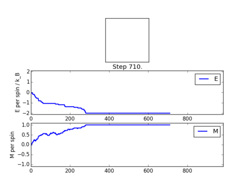
TASK: If $T<T_C$, do you expect a spontaneous magnetisation (i.e. do you expect $⟨M⟩\ne 0$)? When the state of the simulation appears to stop changing (when you have reached an equilibrium state), use the controls to export the output to PNG and attach this to your report. You should also include the output from your statistics() function.

You would expect an spontaneous magnetisation if T is less than T_C as the enthalpic preference for aligned spins is not overcome by thermal excitation. By examining ΔG=ΔH-TΔS we can see that entropic term increases with the temperature of the system, however below the Curie Temperature there is a surplus of spin in one direction for a system at equilibrium.

Results from Ilanmin.py

Screenshot of ILanim.py	Values returned from Statistics function

Accelerating the Code

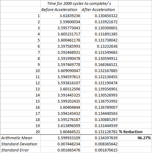
The code was time trialed before and after acceleration. The timetrial was run 20 times before and after modification in order to give an accurate estimate of the mean execution time. These results show a drastic reduction in execution time. It is quite an advantage using a C based extension as opposed to nested for loops!

The effect of Temperature on our Lattices

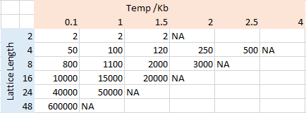
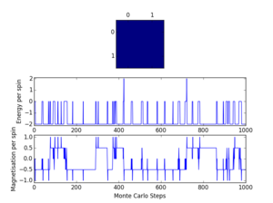
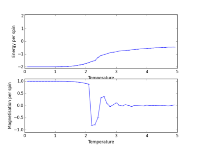
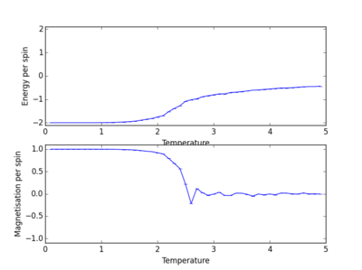
In order to study the effect of temperature of our system we need a method to acquire reliable values for the averages of energy and magnification. This is done by taking the mean value of the attribute over an extended number of cycles when at equilibrium. It is therefore required to ignore the values prior to the equilibrium being achieved. The speed at which equilibrium is established depends on the size of the Ising lattice and also the temperature. Over several runs it was noted that having a larger system size and higher temperature increased the number of cycles required to come to equilibrium. For larger lattices this is because the probability of choosing a spin element that lowers the energy of the system is related to the inverse square of the length of the matrix (we note that the ΔE term is not dependent on lattice size, so can be ignored for comparison of two situations where only the size varies). However, the effect of temperature can be explained by the exp(-ΔE/T) term. As T tends to infinity the exponential function tends to 1, and as T tends to 0 so does the exponential function. Therefore at higher temperatures the system is more likely to accept a spin change that raises the total energy, which means it takes longer to arrive at the equilibrium state from a random distribution. We should also mention that over the Curie Temperature there will be no net magnetisation and that the system equilibrilises about an equal number of randomly distributed spin up/down.

The periods required for the equilibrium were found by repeating ILfinalframe.py 10 times for each temperature/size combination. Reported is an up-rounded approximation of the number of cycles required to reach equilibrium. Selected "typical" figures of "Ilfinalfram.py" are included to evidence this.

Number of cycles required to reach equilibrium

NA- suggests that either the simulation temperature was above the Curie Temperature so no spontaneous magnetisation could occur or equilibrium was not reached in the time scope of this basic investigation.

Typical prints from Ilfinalframe.py

2x2 @ 0.1Kb

2x2 @ 2.5Kb

16x16 @ 1Kb

48x48 @ 0.1Kb

The modification of IsingLattice.py allowed the user to modify the number of cycles that could be discarded before average values began to be calculated. For scanning different temperatures for the largest lattice sizes, a period of discard of 100000 was chosen. This represented a balance between ensuring the lattice could reach equilibrium, whilst also maintaining a realistic calculation time.

Temperature plots for various different lattice sizes

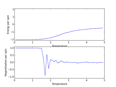
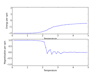
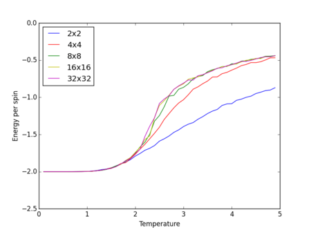
Energy and magnetisation calculations at different temperatures were carried out for various lattice sizes. Each simulation was carried out in the range of 0.1 to 5.0 with a resolution step of 0.1.

Temperature plots from Iltemperaturerange.py

2x2 Lattice	4x4 Lattice
8x8 Lattice	16x16 Lattice
32x32

Combined plots of magnetisation and energy against temperature

Combined Magnetism Plot	Combined Energy Plot

We see from the combined graph of energy per spin against temperature that as the lattice size increases the profile of the curves converge to the same profile. The smallest of the lattices we studied that converges to this profile is the 8x8 system, therefore this is the smallest system to display the long range fluctuations.

Calculating Heat Capacities

The heat capacity of the system can be calculated from the following equation:

$C=\frac{\partial E}{\partial T}=\frac{\mathrm{V}\mathrm{a}\mathrm{r}[E]}{k_B{T}^2}$

The variance can be calculated from subtracting the sum of each value squared from the total sum of the energies squared. This has units of K_B². Noting that T has reduced units of K_B, the units of C must be K_B^-1.

Heat capacity per spin against temperature for various lattice sizes

File:Combined Heat Capacity plots.png

The heat capacity maxima, which correspond to the Schottky anomaly, can be seen to migrate to smaller values for larger lattice sizes.

Locating the Curie Temperature

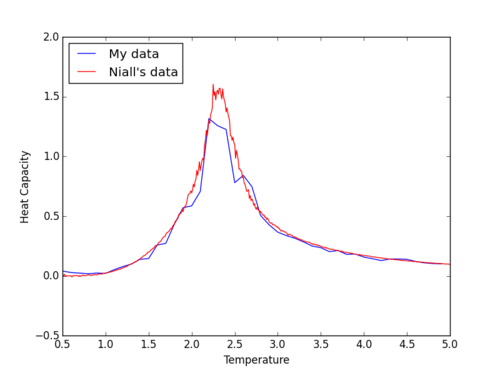
For this part of the experiment we analysed data that had been generated in C++. The step was compare our own generated data to that given. Comparison of the two sets showed relatively strong agreement suggesting that the experimental technique is easily repeatable and reliable.

Comparison of Nas' and Niall's heat capacities of a 16x16 lattice

Relatively good agreement of data. Great detail could be achieved for my results if a smaller temperature step had been used for the calculation.

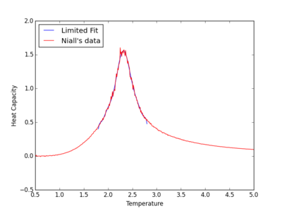
We now needed to fit a polynomial to our results in order to acquire an accurate estimate for the Tc for each lattice. This was first done by fitting a polynomial to the whole range of data which produced a poor match. This was improved by increasing the degree of polynomial used in the fitting process.However a greater improvement could be found by restricting the region of data to be fitted to the peak region. The table below shows a selection of fits with different degrees of polynomials and peak restriction.

C fits for Niall's data on a 16x16 Lattice

3rd Order Fit	3rd Order Fit - peak restriction
6th Order Fit	7th Order - peak restriction
10th Order	10th Order - peak restriction

Using higher order polynomials may be expected to give better fits for the heat capacity. However np.polyval is inaccurate for high order polynomials larger than 10 due to rounding errors in its calculation. Therefore a polynomial of 10 was the maximum used for our fits.

The final step of our study is to determine the Curie temperature of an infinite lattice. This can be done using the following relation:

$T_{C,L}=\frac{A}{L}+T_{C,\mathrm{\infty }}$, where $T_{C,L}$ is the Curie temperature of an $L\times L$lattice, $T_{C,\mathrm{\infty }}$ is the Curie temperature of an infinite lattice, and $A$ is a constant in which we are not especially interested.

Therefore by plotting our Cmaxes for each lattice size against 1/L we can find a best fit line and interpolate the Y intercept, which will be our T_c infinity.

Determination of T_{c infinity}

By calculation we find that Tc infinity = 2.2868351

The value for this reported in literature is 2.269185 . This is relatively good agreement from quite a crude model and demonstrates the power of statistical modelling for physical systems. I was surprised how we were able to replicate published results to good agreement with a very simple approach. The most likely source of error comes from the variable results at the phase transition. This in turn may give an inaccurate value for Cmax for each lattice. This could be improved by running more repeats around the phase transition and also by running many more lattice sizes. This will mean the final best fit line is more accurate, yielding a more accurate result.

References

<references>