Monte Carlo simulation using Ising Model

Introduction

The aim of this computational experiment is to understand the ferromagnetic behaviour using Monte Carlo simulation of a 2D Ising model. The heat capacity and the Curie temperature of the system is also investigated.

Ising model is a mathematical model used in statistical mechanics to depict ferromagnetism. In this model, the atomic spins of either +1 or -1 are arranged in a lattice and the spins are allowed to interact with its neighbours. As the temperature increases from 0K, the system moves from a parallel spin configuration (with a magnetisation of ±N, where N is the number of atoms in the lattice) to an anti-parallel spin configuration with 0 magnetisation. This phenomenon is also known as a phase transition and can be studied using the Monte Carlo simulation.

During this experiment, the Monte Carlo simulation calculates the numerical averages of energies and magnetisation through computational algorithm and random sampling.

Introduction to Ising Model

TASK: Show that the lowest possible energy for the Ising model is $E = - D N J$ , where $D$ is the number of dimensions and $N$ is the total number of spins. What is the multiplicity of this state? Calculate its entropy.

In the Ising model, the interaction energy is given by $- \frac{1}{2} J \sum_{i}^{N} \sum_{j \in n e i g h b o u r s (i)} s_{i} s_{j}$ .

In one dimension, each atom/cell has two neighbours which repeats due to the periodicity of the lattice.

3

1

2

3

From the table above, cell 1 interacts with cell 3 and 2, whereas 2 interacts with 1 and 3. For the lowest energy configuration, the neighbouring cells will have the same spin. Therefore, the interaction energy is given by $- \frac{1}{2} J N (2 s_{i} s_{j})$ , which is equal to $E = - N J$ where D=1. In 2D there are 4 interactions per cell and the lowest energy is given by $E = - 2 N J$ where D=2. Therefore, the lowest possible energy for the Ising model is given by $E = - D N J$ .

In the lowest energy configuration, as all the cells have the same spin, it can be either +1 or -1, giving two possible states. The multiplicity is 2. Entropy is therefore $K_{b} l n 2$ .

TASK: Imagine that the system is in the lowest energy configuration. To move to a different state, one of the spins must spontaneously change direction ("flip"). What is the change in energy if this happens ( $D = 3, N = 1000$ )? How much entropy does the system gain by doing so?

In the lowest energy configuration, the energy of the system is -3000J. When a spin is flipped, firstly the system loses 6 favourable interactions, gaining 6J. Moreover, it then has 6 unfavourable interactions which also adds 6J. In total the energy of the system increases by 12J.

In a system where N=1000, any of the 1000 spins can flip giving 1000 configurations. Therefore entropy is $K_{b} l n (1000)$ .

TASK: Calculate the magnetisation of the 1D and 2D lattices in figure 1. What magnetisation would you expect to observe for an Ising lattice with $D = 3, N = 1000$ at absolute zero?

1D Lattice: +1

2D Lattice: +1

For the 3D Ising Lattice with 1000 cells: At 0K, lowest possible energy configuration with total magnetisation is observed. Therefore the lattice can either have all spins up or spins down. This will give a total magnetisation of ±1000.

Calculating energy and magnetisation

TASK: complete the functions energy() and magnetisation(), which should return the energy of the lattice and the total magnetisation, respectively. In the energy() function you may assume that $J = 1.0$ at all times (in fact, we are working in reduced units in which $J = k_{B}$ , but there will be more information about this in later sections). Do not worry about the efficiency of the code at the moment — we will address the speed in a later part of the experiment.

TASK: Run the ILcheck.py script from the IPython Qt console using the command

%run ILcheck.py

The displayed window has a series of control buttons in the bottom left, one of which will allow you to export the figure as a PNG image. Save an image of the ILcheck.py output, and include it in your report.

The result from ILcheck.py in Fig 1. shows a 4x4 lattices from a low energy state with all parallel spins to a high energy state with alternating anti-parallel spins. This shows the effect of increasing temperature.

Introduction to Monte Carlo simulation

TASK: How many configurations are available to a system with 100 spins? To evaluate these expressions, we have to calculate the energy and magnetisation for each of these configurations, then perform the sum. Let's be very, very, generous, and say that we can analyse $1 \times 1 0^{9}$ configurations per second with our computer. How long will it take to evaluate a single value of ${⟨ M ⟩}_{T}$ ?

For a system with 100 spins, there are 2¹⁰⁰configurations. To evaluate a single ${⟨ M ⟩}_{T}$ value, it would take 1.467x10¹⁶ days. Since it takes so long to compute a single value of magnetisation, Ising model cannot be directly used to calculate energy and magnetisation.

TASK: Implement a single cycle of the above algorithm in the montecarlocycle(T) function. This function should return the energy of your lattice and the magnetisation at the end of the cycle. You may assume that the energy returned by your energy() function is in units of $k_{B}$ ! Complete the statistics() function. This should return the following quantities whenever it is called: $< E >, < E^{2} >, < M >, < M^{2} >$ , and the number of Monte Carlo steps that have elapsed.

Results from montecarlostep() for a 8x8 lattice at T=1.0: (8.0, 2.0)

Results from the statistics() function for a 8x8 lattice at T=1.0 : (8.0, 64.0, 2.0, 4.0, 1)

TASK: If $T < T_{C}$ , do you expect a spontaneous magnetisation (i.e. do you expect $⟨ M ⟩ \neq 0$ )? When the state of the simulation appears to stop changing (when you have reached an equilibrium state), use the controls to export the output to PNG and attach this to your report. You should also include the output from your statistics() function.

$F = U - T S$ , where $F$ is the Helmholtz free energy, $U$ is the internal energy of the system, $T$ is temperature and $S$ is entropy.

At a given temperature, the system controls the balance between the entropically favoured configuration and the energetically favoured configuration. When $T < T_{C}$ , the entropic driving force is not big enough to cause spins to flip to anti-parallel spin configuration. Therefore, a large number of parallel spin configuration and spontaneous magnetisation can be observed below the Curie temperature.

From Fig2. it can be seen that after around 600 steps, the system seems to reach equilibrium.

Accelerating the code

TASK: Use the script ILtimetrial.py to record how long your current version of IsingLattice.py takes to perform 2000 Monte Carlo steps. This will vary, depending on what else the computer happens to be doing, so perform repeats and report the error in your average!

Time Taken(s)	9.646776585	9.098013143	9.025683231	9.186795471	9.219164678
Average time taken(s)	9.235286621
Standard Deviation	0.242235881

TASK: Look at the documentation for the NumPy sum function. You should be able to modify your magnetisation() function so that it uses this to evaluate M. The energy is a little trickier. Familiarise yourself with the NumPy roll and multiply functions, and use these to replace your energy double loop (you will need to call roll and multiply twice!).

    def energy(self):
        "Return the total energy of the current lattice configuration."
        energy = -(np.sum(np.multiply(self.lattice(np.roll(self.lattice(1,0))))))-
        (np.sum(np.multiply(self.lattice(np.roll(self.lattice(1,1))))))
        return energy

    def magnetisation(self):
        "Return the total magnetisation of the current lattice configuration."
        magnetisation=np.sum(self.lattice)
        return magnetisation

TASK: Use the script ILtimetrial.py to record how long your new version of IsingLattice.py takes to perform 2000 Monte Carlo steps. This will vary, depending on what else the computer happens to be doing, so perform repeats and report the error in your average!

With the new code, the average time for Monte Carlo steps to run has decreased by 8.73s.

Time Taken(s)	0.577154774	0.500357554	0.493485749	0.486324092	0.485946439
Average time taken(s)	0.508653721
Standard Deviation	0.038747648

The effect of temperature

TASK: The script ILfinalframe.py runs for a given number of cycles at a given temperature, then plots a depiction of the final lattice state as well as graphs of the energy and magnetisation as a function of cycle number. This is much quicker than animating every frame! Experiment with different temperature and lattice sizes. How many cycles are typically needed for the system to go from its random starting position to the equilibrium state? Modify your statistics() and montecarlostep() functions so that the first N cycles of the simulation are ignored when calculating the averages. You should state in your report what period you chose to ignore, and include graphs from ILfinalframe.py to illustrate your motivation in choosing this figure.

As lattice size and temperature of the system increases, the Monte Carlo steps needed for equilibrium increases. For a 2x2 lattice, at T=5.0, it reached equilibrium before 20,000 steps. However, a 32x32 lattice requires nearly 50,000 steps.

It can be seen from Fig 3. and Fig 4. that 20x20 lattice at a low temperature requires far lesser steps than 50x50 at a higher temperature. In order to not waste computational energy, the minimum number of steps was set to 20,000 without a upper limit. The montecarlostep function was modified so that the monetcarlostep result is only recorded of if the standard deviation is less than 5% of the mean. The code is further explained below. No change was made to the statistics function.

def montecarlostep(self, T):
        energy_list=[]
        self.n_cycles = self.n_cycles + 1
        self.steps=self.steps+1
        energy = self.energy()

        #First montecarlostep is run and the result is added to the energy_list
        random_i = np.random.choice(range(0, self.n_rows))
        random_j = np.random.choice(range(0, self.n_cols))
        self.lattice[random_i,random_j] = -self.lattice[random_i,random_j]
        energy_diff = self.energy() - energy
        random_number = np.random.random()
        if energy_diff > 0:
            if random_number > np.exp(-energy_diff/T):
                self.lattice[random_i,random_j] = -self.lattice[random_i,random_j]
        energy_list=energy_list+[energy]
       
        #More values are added to the energy list by running the monetcarlostep in order to calculate standard deviation
        while (self.steps<20000):
            energy = self.energy()
            #
            random_i = np.random.choice(range(0, self.n_rows))
            random_j = np.random.choice(range(0, self.n_cols))
            self.lattice[random_i,random_j] = -self.lattice[random_i,random_j]
            energy_diff = self.energy() - energy
            random_number = np.random.random()
            #
            if energy_diff > 0:
                if random_number > np.exp(-energy_diff/T):
                    self.lattice[random_i,random_j] = -self.lattice[random_i,random_j]
            energy_list=energy_list+[energy]
            self.steps=self.steps+1

       #To make sure the following step only runs the first time the IF condition is specified
        i=0
        if self.steps==20000:
            #Montecarlostep is run till the standard deviation of the energy list is less than 5% of the mean.
            while i==0:
                if np.std(energy_list)>abs(0.05*np.mean(energy_list)):
                    #
                    random_i = np.random.choice(range(0, self.n_rows))
                    random_j = np.random.choice(range(0, self.n_cols))
                    self.lattice[random_i,random_j] = -self.lattice[random_i,random_j]
                    energy_diff = self.energy() - energy
                    random_number = np.random.random()
                    #this will choose a random number in the range[0,1)
                    if energy_diff > 0:
                        if random_number > np.exp(-energy_diff/T):
                            self.lattice[random_i,random_j] = -self.lattice[random_i,random_j]
                    energy_list=energy_list+[energy]
                    self.steps=self.steps+1
                if np.std(energy_list)<abs(0.05*np.mean(energy_list)):
                    i=1
       #The result from the last monte carlo step is recorded   
        self.E = self.E + self.energy()
        self.M = self.M + self.magnetisation()
        self.E2 = self.E2 + self.energy()**2
        self.M2 = self.M2 + self.magnetisation()**2   
        return(self.energy(), self.magnetisation())

Fig5. 8x8 Lattice results with error bars

Fig6. Error bars after zooming in on Fig 5.

TASK: Use ILtemperaturerange.py to plot the average energy and magnetisation for each temperature, with error bars, for an $8 \times 8$ lattice. Use your intuition and results from the script ILfinalframe.py to estimate how many cycles each simulation should be. The temperature range 0.25 to 5.0 is sufficient. Use as many temperature points as you feel necessary to illustrate the trend, but do not use a temperature spacing larger than 0.5. The NumPy function savetxt() stores your array of output data on disk — you will need it later. Save the file as 8x8.dat so that you know which lattice size it came from.

Temperature spacing was set to 0.01 to effectively capture long range fluctuations. After the montecarlostep is run for the first time for the lattice at a specific temperature, it is already reached the equilibrium value. The runtime was therefore set 100,000 cycles to make sure the average calculated has the smallest standard deviation and standard error possible. Due to this, the error bars being plotted (using standard error) are extremely small and cannot be seen without zooming in.

As temperature increases, energy/spin remains relatively constant at -2.0 till the critical region. Near $T_{c}$ (between T=2.0 and T=3.0), energy/spin increases to 0.0 and remains relatively constant after.

The initial magnetisation is +1 with all parallel spins. As temperature increases close to the $T_{c}$ , the entropic driving force takes over and cause spin flipping to maximise entropy. This creates an anti-parallel spin configuration with equal and alternating spin ups and downs, giving 0 magnetisation.

The effect of system size

TASK: Repeat the final task of the previous section for the following lattice sizes: 2x2, 4x4, 8x8, 16x16, 32x32. Make sure that you name each datafile that your produce after the corresponding lattice size! Write a Python script to make a plot showing the energy per spin versus temperature for each of your lattice sizes. Hint: the NumPy loadtxt function is the reverse of the savetxt function, and can be used to read your previously saved files into the script. Repeat this for the magnetisation. As before, use the plot controls to save your a PNG image of your plot and attach this to the report. How big a lattice do you think is big enough to capture the long range fluctuations?

As the lattice size increases, long range fluctuations decrease. 16x16 is large enough to capture these fluctuations. In the critical region around $T_{c}$ , a single change in spin can have a large impact on magnetisation. In a smaller lattice, the impact of this single spin is greater due to the small number of configurations available for spin flipping. However in a larger lattice, this impact is smaller and therefore fluctuations are also much smaller.

Lattice size	Energy/spin vs Temperature	Magnetisation/spin vs Temperature
2x2
4x4
8x8
16x16
32x32

Determining heat capacity

TASK: By definition,

$C = \frac{\partial ⟨ E ⟩}{\partial T}$

From this, show that

$C = \frac{V a r [E]}{k_{B} T^{2}}$

(Where $V a r [E]$ is the variance in $E$ .)

Expectation of energy or the ensemble energy average is given by the sum of the microstate energy $E_{i}$ times its probability $P_{i}$ .

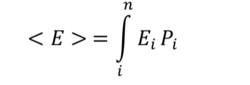
The previous equation can therefore be written in terms of the partition function $Z$ : , where .

When <E> is differentiated with respect to T, we obtain the following equation:

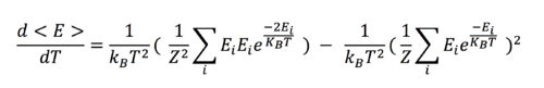
Upon further simplification: .

Also, .

Therefore, .

TASK: Write a Python script to make a plot showing the heat capacity versus temperature for each of your lattice sizes from the previous section. You may need to do some research to recall the connection between the variance of a variable, $V a r [X]$ , the mean of its square $⟨ X^{2} ⟩$ , and its squared mean ${⟨ X ⟩}^{2}$ . You may find that the data around the peak is very noisy — this is normal, and is a result of being in the critical region. As before, use the plot controls to save your a PNG image of your plot and attach this to the report.

As lattice size increases, the graph becomes narrower and noisier around the critical region. The maximum heat capacity value increases with increasing lattice size from approximately 0.1 to 1.5.

Lattice size	Heat capacity/spin vs Temperature
2x2
4x4
8x8
16x16
32x32

Locating the Curie temperature

TASK: A C++ program has been used to run some much longer simulations than would be possible on the college computers in Python. You can view its source code here if you are interested. Each file contains six columns: $T, E, E^{2}, M, M^{2}, C$ (the final five quantities are per spin), and you can read them with the NumPy loadtxt function as before. For each lattice size, plot the C++ data against your data. For one lattice size, save a PNG of this comparison and add it to your report — add a legend to the graph to label which is which. To do this, you will need to pass the label="..." keyword to the plot function, then call the legend() function of the axis object (documentation here).

Lattice size	32x32	Comment
Energy/spin vs Temperature		C++ data and python data are very similar. However the python data has more fluctuations this maybe due to the fact that the runtime in the python simulation was smaller than C++, thereby producing more fluctuations.
Magnetisation/spin vs Temperature		Magnetisation in C++ data goes to zero before python data. This might be due to smaller temperature spacing in the C++ run which accurately captures the critical region causing the magnetisation to quickly drop to 0.
Heat Capacity/spin vs Temperature		C++ Heat Capacities produce a narrower peak with lesser fluctuations than python. This can again be attributed to runtime and temperature spacing.

Fig23. Initial polynomial fitting for 4x4 lattice.

TASK: write a script to read the data from a particular file, and plot C vs T, as well as a fitted polynomial. Try changing the degree of the polynomial to improve the fit — in general, it might be difficult to get a good fit! Attach a PNG of an example fit to your report.

It is difficult to get a good fit across the whole plot as the plot is not strictly polynomial. The degree of polynomial fitting was increases to very high values such as 9 and 11 to get a good fitting throughout the plot. However because of this high degree, the fitting may not be reliable over the whole region and cannot be used to extrapolate data.

#first we fit the polynomial to the data
fit = np.polyfit(T4, H4, 9) # fit a third order polynomial

#now we generate interpolated values of the fitted polynomial over the range of functions
T4_min = np.min(T4)
T4_max = np.max(T4)
T_range4 = np.linspace(T4_min, T4_max, 10000) #generate 1000 evenly spaced points between T_min and T_max
fitted_C4_values = np.polyval(fit, T_range4) # use the fit object to generate the corresponding values of C
plot(T4, H4 , label = "Initial Heat Capacity")
plot(T_range4, fitted_C4_values, label = "Fitted Heat Capacity")
legend()
title("Fitting of Heat Capacity for 4X4 lattice")
xlabel("Temperature")
ylabel("Heat Capacity")
show()

Fig24.Polynomial fitting of the peak for 4x4 lattice.

TASK: Modify your script from the previous section. You should still plot the whole temperature range, but fit the polynomial only to the peak of the heat capacity! You should find it easier to get a good fit when restricted to this region.

The fitting was limited to the region between T=2.0 and T=3.0. This fitting gives a good plot and reliable data in the critical region.

def fitting_HC(T2,H2,T2_min,T2_max,n):
    new_temp=[]
    new_C=[]
    T2_min = 2 
    T2_max = 3 
    i=0

    min_temp_selection = np.logical_and(T2 < T2_min, i==i )
    min_T2_values = T2[min_temp_selection]
    min_H2_values = H2[min_temp_selection]
    new_temp=new_temp+list(min_T2_values)
    new_C=new_C+list(min_H2_values)

    selection = np.logical_and(T2 > T2_min, T2 < T2_max) #choose only those rows where both conditions are true
    peak_T2_values = T2[selection]
    peak_H2_values = H2[selection]

    fit = np.polyfit(peak_T2_values, peak_H2_values, 3) 

    T_range2 = np.linspace(T2_min, T2_max, 1000) #generate 1000 evenly spaced points between T_min and T_max
    fitted_C2_values = np.polyval(fit, T_range2) # use the fit objectto generate the corresponding values of C

    new_temp=new_temp+list(T_range2)
    new_C=new_C+list(fitted_C2_values)

    max_temp_selection = np.logical_and(T2 > T2_max,i==i)
    max_T2_values = T2[max_temp_selection]
    max_H2_values = H2[max_temp_selection]
    new_temp=new_temp+list(max_T2_values)
    new_C=new_C+list(max_H2_values)
    
    plot(new_temp, new_C, label = "Fitted Heat Capacity")
    legend()
    xlabel("Temperature")
    ylabel("Heat Capacity")
    title("Fitting of Heat Capacity for "+str(n)+' lattice')
    return

TASK: find the temperature at which the maximum in C occurs for each datafile that you were given. Make a text file containing two colums: the lattice side length (2,4,8, etc.), and the temperature at which C is a maximum. This is your estimate of $T_{C}$ for that side length. Make a plot that uses the scaling relation given above to determine $T_{C, \infty}$ . By doing a little research online, you should be able to find the theoretical exact Curie temperature for the infinite 2D Ising lattice. How does your value compare to this? Are you surprised by how good/bad the agreement is? Attach a PNG of this final graph to your report, and discuss briefly what you think the major sources of error are in your estimate.

Fig23.Polynomial fitting of the peak for 4x4 lattice.

$T_{C, \infty}$ was calculated to be 2.288¹ $J / k_{b}$ . The literature $T_{C, \infty}$ is 2.269 $J / k_{b}$ . The percentage difference is 0.837% which is extremely small. This shows that the fitting is very good and that the results by comparing relatively smaller lattices still give a reliable value for $T_{C, \infty}$ .

However, from the graph it can be seen that the linear fitting is not very good as the data does not show a strong linear correlation. Repeats must be taken to improve fitting.

The major source of error is from using a maximum lattice size of 32x32 which is still small to compute $T_{C, \infty}$ . The smaller lattices do not accurately depict the infinite lattice as the number of configurations in a 32x32 lattice is much smaller. Computing this simulation for larger lattices will improve the accuracy of $T_{C, \infty}$ .

Moreover, In ILtemperaturerange.py, the runtime for each lattice size can be increased to further reduce the error (standard deviation) in the computed energy and magnetisation values, which will in turn reduce the error in the $T_{C, \infty}$ calculated.

Conclusion

In conclusion, the Monte Carlo simulation of the Ising model even at smaller lattice sizes provides a accurate and reliable depiction of ferromagnetism and phase transition. The phase transition is observed at T=2.288 which is in agreement with the analytical data, with only a small percentage difference.

Further experiments can be also be carried out to better test the efficacy of Monte Carlo simulation and the Ising Model:

The simulation can be carried out in 3D, using a 3D Ising model to predict phase transition in 3D structures such as crystals and metals.
Can modify the force coupling parameter , J² , to be distance dependent to model the actual force field (like Lennard-Jones potential) in a metal or crystal.

References

Onsager, Lars (1944), "Crystal statistics. I. A two-dimensional model with an order-disorder transition", Phys. Rev. (2) 65(3–4): 117–149
Markov Processes, Gillespie, 4^thedn