Rep:Molecular Dynamics RS7913

Mainly quite good - you need to mature your writing style but well written. ALthough your radial distribution function for liquid and gas is not correct, everything else is and your explanation for heat capacity is good. Mark: 69/100

Abstract

This is quite good - should put some of your data in here to back up your critical statements (i.e. your diffusion coefficients).

The LAMMPS molecular dynamics package was used to determine the mean squared displacement (MSD) and velocity autocorrelation functions (VACF) for a monatomic Lennard-Jones solid, liquid and gas, from which the corresponding diffusion coefficients were calculated. Whilst both methods gave rise to similar relative diffusion coefficients for the solid, liquid and gaseous systems, the absolute values given by the two methods differed by between six and ten orders of magnitude when comparing the results obtained using the two different functions to modelling the same system. It is suspected that using the MSD results in a more accurate estimation of diffusion coefficient due to the additional source of error when using the VACFs to do so, which is the use of the trapezium rule.

Introduction

As we discussed, you should target your audience in your introduction - find some interesting literature and work with that.

Computational molecular dynamics simulations provide a simple and fast method of calculating thermodynamic properties without having to carry out practical work in the laboratory, and is especially useful when modelling systems such as biological systems, for which it may be difficult to make models in the lab. Such methods can be used to calculate diffusion coefficients of various systems. The diffusion coefficient is an important thermodynamic quantity that can be useful to consider when investigating a wide range of phenomena such as the electrolysis of some substance the phrase 'some substance' is too colloquial, to the movement of atoms or molecules (e.g. drug molecules) around the human body.

Employing a Lennard-Jones model to calculate thermodynamic properties is very useful since Lennard-Jones parameters exist for many different systems, and the results obtained can be used to gain information about a wide range of systems, from a bulk metal to argon gas. In this investigation, the LAMMPS molecular dynamics package was used to model a monatomic Lennard-Jones solid, liquid and gas.

Aims and Objectives

Also to calculate equation of state and heat capacity but good

• To determine the diffusion coefficients for a monatomic Lennard-Jones solid, liquid and gas using the MSD function.
• To determine the diffusion coefficients for a monatomic Lennard-Jones solid, liquid and gas using the VACF.
• To rationalise the MSD functions and VACFs calculated.
• To compare and contrast the use of the two methods for calculating these diffusion coefficients, and determine which is a more suitable and more accurate method.

Methods

Structure this section model-forcefield-techniques. We've used a few throughout the experiment so section these.

The LAMMPS molecular dynamics package was used with the forcefield set to Lennard-Jones with a cutoff of 3.2σ, and pairwise coefficients set to 1.0, 1.0. Simulations were run for a vapour (density = 0.05, initialised as a sc lattice), liquid (density = 0.8, initialised as a sc lattice) and solid (density = 1.2, with lattice type set to fcc), at a reduced temperature of 1.0. Systems containing 8000 atoms (20x20x20 grid) and 1000000 (100x100x100 grid) were simulated in the NVT ensemble. Microsoft Excel was used to carry out subsequent data analysis on the results from the MD simulations.

Results and Discussion

Using the mean squared displacement to calculate the diffusion coefficient

The total MSD as a function of timestep for the solid, liquid and gas simulations carried out with N = 8000 and N = 1000000 were plotted, and a linear fit has been applied to each of these functions.

Figure 1: MSD as a function of timestep for the gas simulations, with the linear fits shown.

Figure 2: MSD as a function of timestep for the liquid simulations, with the linear fits shown.

Figure 3: MSD as a function of timestep for the solid simulations, with the linear fits shown.

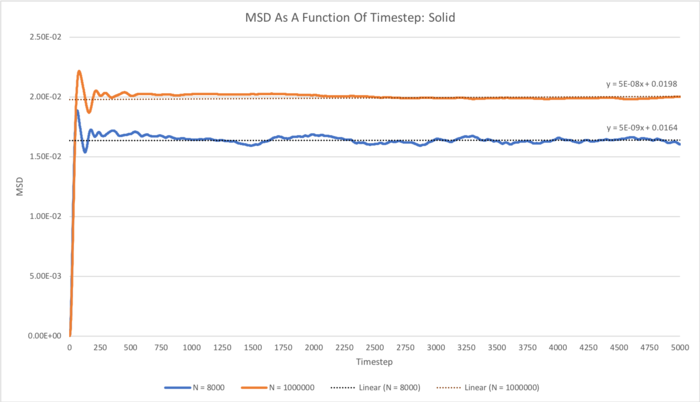
would be nice for you to derive the power law here -> msd α t^a

In the case of the liquid, excellent linear behaviour is maintained throughout the simulation, as would be expected for the random Brownian motion in the system. However, in the solid and gas phases, it does require some time for linear behaviour to be established, and this could be attributed to the time required for the ballistic/diffusive regimethat fade away, which can be thought of as anisotropic 'vibrations' in the system due to molecules in the ordered FCC lattice colliding backwards and forwards with one another over and over again, spreading the kinetic energy over the whole solid until equilibrium is reached, and the system does equilibrate relatively quickly. The MSD function for the gas phase, however, initially has an upwards curvature, indicating some sort of external force acting on the particles. The positive curvature in fact indicates that we are looking at the ballistic regime, which occurs in the gaseous phase since the density is so low that the atoms having a relatively long mean free path length. The gradient of the MSD for the gaseous calculations were only measured by considering the subsequent linear region into account - the diffusive regime - from around timestep 2250 onwards. Since this part of the function corresponds to the true random motion of particles in the system, it can therefore be used to calculate the diffusion coefficient of the system with adequate accuracy.

As expected, the gradient was greatest for the gas, followed by the liquid, whereas the gradient for the solid phase was essentially zero. This is because particles in the gas phase move the most (due to the lower density meaning movement of particles is not constricted by collisions), followed by those in the liquid. The fact that the solid function is essentially flat reflects the fact that the particles do not have net movement in the solid, but only some oscillations backwards and forwards at the beginning of the simulation as mentioned.

In the case of the liquid and gas simulations, increasing the size of the system from 8000 to 1000000 atoms doesn't seem to result in any great qualitative difference in terms of the MSD. However, in the case of the solid simulation it can clearly be seen that the MSD flattens out to a virtually straight line in the 1000000-atom simulation, whereas for the 8000-atom simulation, the function does not really completely flatten out over the course of the simulation, indicating that this smaller system size may not be quite large enough to gain accurate information in terms of the MSD. A larger-scale simulation of some system containing a greater number of particles will of course inherently result in better statistical information in each frame assessed compared to a smaller-scale simulation containing fewer particles.

The diffusion coefficient, D, was estimated by dividing the gradient of the linear fit by 6:

	Diffusion Coefficient / σ/√(ε/m*)
Phase	N = 8000	N = 1000000
Solid	8.3333 x 10-9	8.3333 x 10-10
Liquid	1.6667 x 10-4	1.6667 x 10-4
Gas	6.3333 x 10-3	6.0833 x 10-3

Table 1: Diffusion coefficients calculated using the MSD functions.

As expected, the diffusion coefficient is greatest for the gas and lowest for the liquid. The diffusion coefficient for the gas is just under one and a half orders of magnitude greater than that of the liquid, and roughly six orders of magnitude greater than that for the solid. tick, good

Using the velocity autocorrelation function to calculate the diffusion coefficient

C(τ) was plotted as a function of time (timestep (τ), between 0 and 5000) for the Lennard-Jones solid, liquid and gaseous simulations carried out with N set to 8000 and 1000000 atoms in Figures 3 and 4, respectively.

Figure 3: VACF as a function of timestep for the solid, liquid and gaseous simulations carried out with N set to 8000.

Figure 4: VACF as a function of timestep for the solid, liquid and gaseous simulations carried out with N set to 1000000.

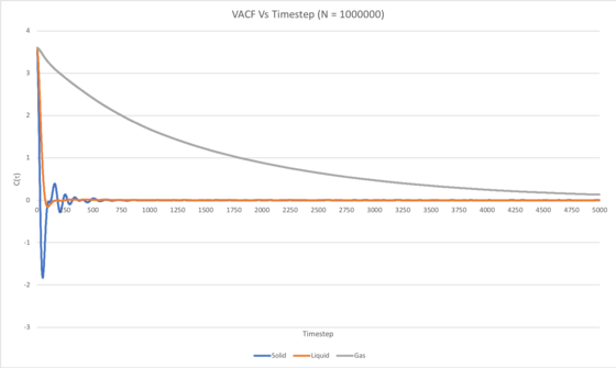
In the case of the liquid and solid systems, the VACF quickly decays to a minimum, which can be thought of as occurring due to all particles in the system having collided. The minimum for the solid system is more pronounced than that for the liquid simulation because the atoms in the solid system form a more ordered FCC lattice, hence the particles will collide in a uniform fashion to give a clear, more definite negative correlation once all the particles in the system have collided. The minimum for the solid system also occurs more quickly (i.e. at an earlier timestep) in comparison to the liquid simulation, and this may be attributed to the greater density of the solid system resulting in more frequent collisions and therefore all of the particles having collided in a shorter timeframe. Also, a number of oscillations can be seen in the VACF of the Lennard-Jones solid, and this corresponds to the velocities of the atoms in the system fluctuating between being positively and negatively correlated to their initial velocities. This can essentially be thought of as the atoms in the system 'vibrating' as they collide back and forth between neighbouring atoms, since the structure is an ordered FCC lattice. This of course occurs until the kinetic energy has been dissipated evenly between all atoms in the solid, at which point the VACF has decayed to a constant value of 0. Three weak oscillations can be seen in the VACF of the Lennard-Jones liquid, and this is due to a similar collision of atoms forwards and backwards as in the solid, but in this case is caused by the short-range order in the liquid.

For the 1000000-atom liquid and solid simulations, it can be seen that the VACF decays to a constant value of 1, however the corresponding VACFs for the 8000-atom simulation continually fluctuates by a small amount throughout the course of the simulation, even once the function has decayed. This may indicate that an 8000-atom simulation is not sufficiently large for calculation of an adequately accurate VACF for a monatomic Lennard-Jones solid or liquid.

It takes considerably longer for the VACF to decay to the constant value of 0 in the gaseous simulation in comparison to that of the solid and liquid, for which the VACF decays quite quickly, due to the far lower density of the gas.

The trapezium rule was used to approximate the integral under the VACF, using a function that created trapezia of 1 timestep 'width'.

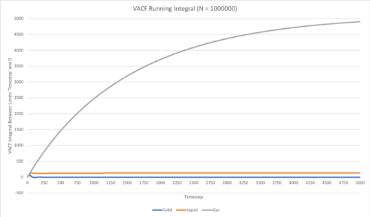
Figure 5 (left): Running integrals for the solid, liquid and gas simulations carried out with N set to 8000 atoms. Figure 6 (right): Running integrals for the solid, liquid and gas simulations carried out with N set to 1000000 atoms.

As can be seen in Figures 5 and 6, in all cases the running integral converges to a constant value over the duration of the simulation, as expected. It takes considerably longer for this to occur in the gaseous simulation in comparison to that of the solid and liquid, for which the running integral converges quite quickly. This is due to the far lower density of the gas meaning the frequency of collisions in the system is much lower than that in the case of the solid and liquid simulations, therefore the time taken for the kinetic energy to be evenly distributed over all atoms in the system is far greater, thus the time taken for the VACF to decay to the constant value of 0 is considerably longer, as can be seen in Figures 3 and 4. Indeed, in the case of the gaseous simulation with N set to 1000000 atoms (see Figure 4), the VACF had not fully decayed within the timeframe of the simulation, therefore the running integral had not completely converged. Hence, would be worthwhile to repeat this particular simulation for a slightly longer duration to gain more accurate information in terms of the diffusion coefficient.

D was calculated using the by dividing the integral of C(τ) over all τ (0 to 5000) by 3:

	Diffusion Coefficient / σ/√(ε/m*)
Phase	N = 8000	N = 1000000
Solid	0.060364158	0.022764742
Liquid	34.47327454	45.04573814
Gas	1089.389257	1634.232899

Table 1: Diffusion coefficients calculated using the VACFs.

It can be seen that the diffusion coefficient (D) for the gas is just under 2 orders of magnitude greater than that of the liquid, and roughly four and a half orders of magnitude greater than that for the solid. This relative trend is what would be expected in terms of D for a solid, liquid and gas, and is somewhat similar to that calculated using the MSD, however the absolute values of D calculated using the VACFs are far greater than those calculated using the MSDs. Use of the trapezium rule (underestimates the area under maxima and overestimates the area under minima in a graph) when using the VACFs to calculate diffusion coefficients is an additional source of error that arises that is not a factor when using the MSD to calculate D, and could likely be the greatest source of error when estimating diffusion coefficients from the VACFs. Other sources of error in the estimations of D carried out could be use of the Lennard-Jones cutoff of 3σ, however this cutoff is quite standard when carrying out these kinds of simulations in research, and usually results in relatively accurate simulations of model systems in the literature. In addition, it is important that the Lennard-Jones model is indeed a good enough model for the system under investigation, otherwise the results obtained would not be appropriate. It is worth noting that these last two potential sources of error concerning the Lennard-Jones cutoff and appropriate use of the Lennard-Jones model itself is applicable to both calculations of D using the MSD and VACF methods.

Conclusion

Whilst using both the MSD and VACF functions to calculate the diffusion coefficients for a monatomic system of a Lennard-Jones solid, liquid and gas will result in reasonable relative values of D for the solid, liquid and gaseous systems when considering one method at a time, there are some flaws. Using the MSD functions to calculate the diffusion coefficients resulted in absolute values that were around six orders of magnitude smaller than those same diffusion coefficients calculated using the VACFs. This discrepancy is far too great to be considered as negligible, and it would be useful to look at the Lennard-Jones parameters for some monatomic systems and see how the diffusion coefficients calculated actually compare to those determined by practical investigation in the lab. Such an investigation would allow for a definitive answer as to which method is more accurate for calculating the diffusion coefficient, as well as how the size of the system simulated, N, affects the accuracy of the estimated diffusion coefficients. Indeed, varying the timestep and duration of the simulation, as well examining systems even larger than 1000000 atoms, would also be useful subjects of further research.

Whilst it cannot be definitively concluded which method is better for calculating the diffusion coefficient for a monatomic Lennard-Jones system based solely on the investigation carried out here, it would be expected that using the MSD functions would result in the more accurate results. This is because use of the trapezium rule to calculate the VACF integrals is an additional source of error that does not apply to use of the MSD functions to calculate diffusion coefficients, and likely gives rise to significant error in the calculations carried out.

Tasks

TASK: Open the file HO.xls. In it, the velocity-Verlet algorithm is used to model the behaviour of a classical harmonic oscillator. Complete the three columns "ANALYTICAL", "ERROR", and "ENERGY": "ANALYTICAL" should contain the value of the classical solution for the position at time $t$, "ERROR" should contain the absolute difference between "ANALYTICAL" and the velocity-Verlet solution (i.e. ERROR should always be positive -- make sure you leave the half step rows blank!), and "ENERGY" should contain the total energy of the oscillator for the velocity-Verlet solution. Remember that the position of a classical harmonic oscillator is given by $x\left(t\right)=A\cos (\omega t+\varphi )$ (the values of $A$, $\omega$, and $\varphi$ are worked out for you in the sheet).

See "Analytical" tab in HO_RS7913.xls

TASK: For the default timestep value, 0.1, estimate the positions of the maxima in the ERROR column as a function of time. Make a plot showing these values as a function of time, and fit an appropriate function to the data.

See "Analytical" tab in HO_RS7913.xls

TASK: Experiment with different values of the timestep. What sort of a timestep do you need to use to ensure that the total energy does not change by more than 1% over the course of your "simulation"? Why do you think it is important to monitor the total energy of a physical system when modelling its behaviour numerically?

A timestep of 0.2 is just about short enough to ensure that the total energy doesn't change by more than 1% over the course of the simulation, since it results in the total energy oscillating between 0.5 and 0.495. The total energy of this simple harmonic oscillator was calculated by summing the kinetic energy (calculated using the velocity from the velocity-Verlet solution) and the potential energy (calculated using the classical simple harmonic motion equation to calculate the force, F = -kx). In a simple harmonic oscillator, the total energy of the system remains constant as kinetic and potential energy are interchanged. It is important to monitor the total energy of a physical system such as this because the amount by which the total energy varies corresponds to the accuracy of the simulation. Of course, the more accurate the approximation, the smaller the amount by which the energy will vary, and a smaller timestep will result in a more accurate approximation.

See "Timestep" tab in HO_RS7913.xls

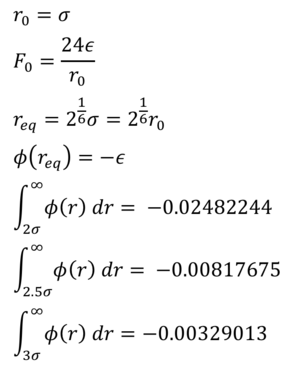
TASK: For a single Lennard-Jones interaction, $\varphi \left(r\right)=4ϵ(\frac{{\sigma }^{12}}{r^{12}}-\frac{{\sigma }^6}{r^6})$, find the separation, $r_0$, at which the potential energy is zero. What is the force at this separation? Find the equilibrium separation, $r_{eq}$, and work out the well depth ($\varphi \left(r_{eq}\right)$). Evaluate the integrals $\underset{2\sigma }{\overset{\mathrm{\infty }}{\int }}\varphi \left(r\right)\mathrm{d}r$, $\underset{2.5\sigma }{\overset{\mathrm{\infty }}{\int }}\varphi \left(r\right)\mathrm{d}r$, and $\underset{3\sigma }{\overset{\mathrm{\infty }}{\int }}\varphi \left(r\right)\mathrm{d}r$ when $\sigma =ϵ=1.0$.

TASK: Estimate the number of water molecules in 1ml of water under standard conditions. Estimate the volume of $10000$ water molecules under standard conditions.

TASK: Consider an atom at position $(0.5,0.5,0.5)$ in a cubic simulation box which runs from $(0,0,0)$ to $(1,1,1)$. In a single timestep, it moves along the vector $(0.7,0.6,0.2)$. At what point does it end up, after the periodic boundary conditions have been applied?

(0.5, 0.5, 0.5) + (0.7, 0.6, 0.2) = (0.2, 0.1, 0.7)

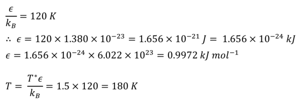
TASK: The Lennard-Jones parameters for argon are $$\begin{gathered} \sigma =0.34\mathrm{n}\mathrm{m},ϵ \\ / \\ {k}_B=120\mathrm{K} \end{gathered}$$. If the LJ cutoff is $r^{*}=3.2$, what is it in real units? What is the well depth in $$\begin{gathered} {\mathrm{k}\mathrm{J} \\ \mathrm{m}\mathrm{o}\mathrm{l}}^{-1} \end{gathered}$$? What is the reduced temperature $T^{*}=1.5$ in real units?

TASK: Why do you think giving atoms random starting coordinates causes problems in simulations? Hint: what happens if two atoms happen to be generated close together?

If random starting coordinates were given to the atoms, two or more atoms may be generated very close to one another. This would mean that these atoms would experience a very strong repulsive force between one another, as given by the Lennard-Jones potential, since the '1/r¹²' term dominates at shorter distance. Hence, the system may not reach equilibrium by the time the simulation has run - although increasing the length of time a simulation is run would increase the chance of the system reaching equilibrium, this would be of computational cost.

TASK: Satisfy yourself that this lattice spacing corresponds to a number density of lattice points of $0.8$. Consider instead a face-centred cubic lattice with a lattice point number density of 1.2. What is the side length of the cubic unit cell?

p = m/v

Volume of a lattice point = (1.07722)³

Therefore, number density of lattice points = 1/(1.07722)³ = 0.8

Face-centered cubic (FCC) lattice contains 4 lattice points within the unit cell

Therefore, the volume of one lattice point = 4/1.2

Side length of FCC unit cell = (4/1.2)^1/3 = 1.49380

TASK: Consider again the face-centred cubic lattice from the previous task. How many atoms would be created by the create_atoms command if you had defined that lattice instead?

The create_atoms command created 1000 atoms for the simple cubic lattice, for which each unit cell contains 1 atom. Since the FCC unit cell contains 4 atoms, the create_atoms command would have created 1000 x 4 = 4000 atoms if this lattice had been defined instead.

TASK: Using the LAMMPS manual, find the purpose of the following commands in the input script:

mass 1 1.0
pair_style lj/cut 3.0
pair_coeff * * 1.0 1.0

"mass 1 1.0" sets the mass of atom type 1 to 1.0

"pair_style lj/cut 3.0" sets the formula used to calculate pairwise interactions between atoms as that defined by the Lennard-Jones potential, with a cutoff of r* = 3.0 

"pair_coeff * * 1.0 1.0" sets the forcefield coefficients - in this case the Lennard-Jones parameters σ and ε - to 1.0

TASK: Given that we are specifying ${\mathbf{x}}_i\left(0\right)$ and ${\mathbf{v}}_i\left(0\right)$, which integration algorithm are we going to use?

We are using the velocity-Verlet algorithm, since the starting positions of the atoms (${\mathbf{x}}_i\left(0\right)$) and their velocities at the same time (${\mathbf{v}}_i\left(0\right)$) must be defined when using the velocity-Varlet. When using the Verlet algorithm, the starting positions of the atoms (${\mathbf{x}}_i\left(0\right)$) and their positions one timestep in the past (${\mathbf{x}}_i(-\delta t)$) must be defined.

TASK: Look at the lines below.

### SPECIFY TIMESTEP ###
variable timestep equal 0.001
variable n_steps equal floor(100/${timestep})
timestep ${timestep}

### RUN SIMULATION ###
run ${n_steps}
run 100000

The second line (starting "variable timestep...") tells LAMMPS that if it encounters the text ${timestep} on a subsequent line, it should replace it by the value given. In this case, the value ${timestep} is always replaced by 0.001. In light of this, what do you think the purpose of these lines is? Why not just write:

timestep 0.001
run 100000

This allows for the timestep to be easily modified by modifying the value "${timestep}", and other sections of the script can also be linked to "${timestep}" to ensure that the timestep for all these sections of the script is set to the desired "${timestep}" value.

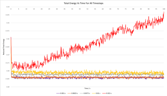
TASK: make plots of the energy, temperature, and pressure, against time for the 0.001 timestep experiment (attach a picture to your report). Does the simulation reach equilibrium? How long does this take? When you have done this, make a single plot which shows the energy versus time for all of the timesteps (again, attach a picture to your report). Choosing a timestep is a balancing act: the shorter the timestep, the more accurately the results of your simulation will reflect the physical reality; short timesteps, however, mean that the same number of simulation steps cover a shorter amount of actual time, and this is very unhelpful if the process you want to study requires observation over a long time. Of the five timesteps that you used, which is the largest to give acceptable results? Which one of the five is a particularly bad choice? Why?

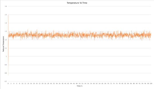
Plots of the total energy, temperature, and pressure, against time for the 0.001 timestep experiment are shown below. It can be seen that the simulation reaches equilibrium at around 0.5 s, after which the total energy oscillates about the average equilibrium value.

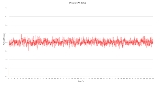
The total energy against time for all timesteps has also been plotted above (bottom right graph). It is clear that the average total energy for the experiments carried out using time steps of 0.001 s and 0.0025 s were very similar; the total energy for both of these experiments oscillated about virtually the same average equilibrium value. The 0.0075 s and 0.01 s timestep experiments both reached equilibrium, however the average energy at equilibrium was considerably greater for the 0.0075 s experiment and even greater for the 0.01 s experiment, and this is indicative that using these experiments are not as accurate. In addition, the amount by which the total energy oscillated once equilibrium was reached was greater for the 0.0075 s experiment and even greater for the 0.01 s experiment, further testifying that these simulations were not as accurate. In the case of the 0.015 s timestep, the simulation did not even reach equilibrium over the duration of the simulation; the energy just continued increasing further and further. This 0.015 s timestep simulation is clearly not accurate, and using such a large timestep is a particularly bad choice. Whilst using the 0.001 s timestep would give the most accurate results, the 0.0025 s timestep is sufficiently short to give acceptable results since the average total energies from both of these calculations are virtually the same. Using a timestep greater than 0.0025 s would likely give inaccurate results.

TASK: Choose 5 temperatures (above the critical temperature $T^{*}=1.5$), and two pressures (you can get a good idea of what a reasonable pressure is in Lennard-Jones units by looking at the average pressure of your simulations from the last section). This gives ten phase points — five temperatures at each pressure. Create 10 copies of npt.in, and modify each to run a simulation at one of your chosen $(p,T)$ points. You should be able to use the results of the previous section to choose a timestep. Submit these ten jobs to the HPC portal. While you wait for them to finish, you should read the next section.

Timestep of 0.0025 chosen

T = 2, 3.5, 5, 6.5, 8

p = 2.5, 3

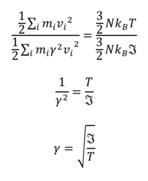
TASK: We need to choose $\gamma$ so that the temperature is correct $T=\mathfrak{𝔗}$ if we multiply every velocity $\gamma$. We can write two equations:

$\frac{1}{2}\sum _i{m}_i{v}_i^2=\frac{3}{2}N{k}_{B}T$

$\frac{1}{2}\sum _i{m}_i{\left(\gamma v_i\right)}^2=\frac{3}{2}N{k}_B\mathfrak{𝔗}$

Solve these to determine $\gamma$.

TASK: Use the manual page to find out the importance of the three numbers 100 1000 100000. How often will values of the temperature, etc., be sampled for the average? How many measurements contribute to the average? Looking to the following line, how much time will you simulate?

The number 100 sets the Nevery variable, which is the number of timesteps between which each sample of the (thermodynamic) data is taken.

The number 1000 sets the Nrepeat variable, which is the number of timesteps between which averages of this sampled data (set by Nevery) are taken.

The number 100000 sets the Nfreq variable, which is the number of timesteps over which an average of the previous averages (determined by Nrepeat) are taken.

The following line "run 100000" instructs LAMMPS to run the simulation over 100000 timesteps. Hence, setting the Nfreq variable to 100000 as done for this simulation essentially instructs LAMMPS to take an average over the whole course of the simulation.

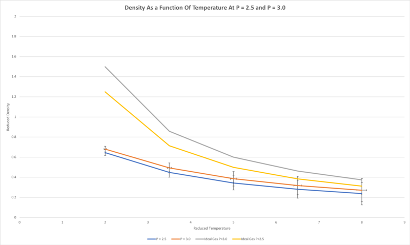
TASK: When your simulations have finished, download the log files as before. At the end of the log file, LAMMPS will output the values and errors for the pressure, temperature, and density $\left(\frac{N}{V}\right)$. Use software of your choice to plot the density as a function of temperature for both of the pressures that you simulated. Your graph(s) should include error bars in both the x and y directions. You should also include a line corresponding to the density predicted by the ideal gas law at that pressure. Is your simulated density lower or higher? Justify this. Does the discrepancy increase or decrease with pressure?

The simulated density, at both reduced pressures of 2.5 and 3.0, was lower than that predicted by the ideal gas law. This is because the ideal gas law models the atoms as simply hard spheres, meaning the atoms cannot get as close to one another as in the molecular dynamics simulations carried out, in which the Lennard-Jones potential is used to model intermolecular interactions. This function is a more accurate representation of the true intermolecular interactions, and accounts for the more gradual onset of repulsion between two atoms as they are brought closer together, caused by electrostatic repulsion between the outer electrons - the deformability of atoms is not accounted for by the ideal gas law. This discrepancy increases with increasing pressure since, at higher pressure, the particles spend more time closer to one another, and bump into one another more often, therefore the deformability of atoms accounted for in the molecular dynamics simulation becomes more significant relative to the ideal gas law hard sphere model.

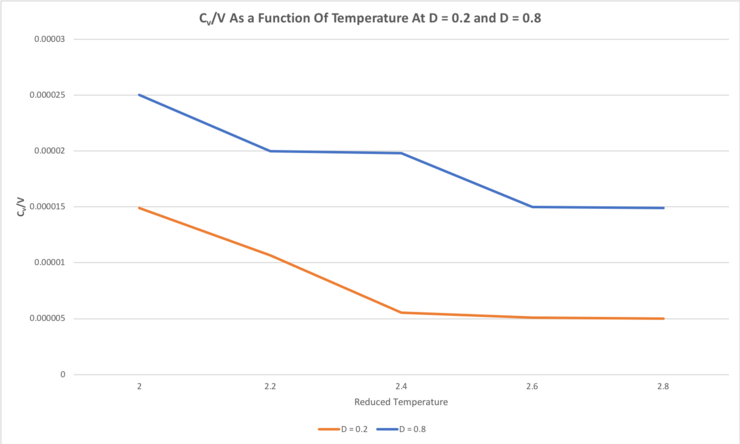
TASK: As in the last section, you need to run simulations at ten phase points. In this section, we will be in density-temperature $({\rho }^{*},T^{*})$ phase space, rather than pressure-temperature phase space. The two densities required at $0.2$ and $0.8$, and the temperature range is $2.0,2.2,2.4,2.6,2.8$. Plot $C_V/V$ as a function of temperature, where $V$ is the volume of the simulation cell, for both of your densities (on the same graph). Is the trend the one you would expect? Attach an example of one of your input scripts to your report.

For both densities of 0.2 and 0.8, the heat capacity at constant volume, C_v, decreases with increasing temperature. This trend would not be expected; the heat capacity per unit volume should remain constant with respect to temperature because the inherent chemical properties of the system have not changed. Since both the density and volume - because we are considering the heat capacity of some unit volume V (C_v/V) - are fixed, the number of particles being considered does not change as the temperature is varied, hence the internal energy remains constant. Since the heat capacity at constant volume can be defined as C_v = dU/dT, the fact that the internal energy remains constant as the temperature is varied inherently means that the heat capacity also remains constant as the temperature is varied.

The heat capacity, C_v, also increases with increasing density, which would be the expected trend. Since we are considering the heat capacity of some unit volume (V) of the system (C_v/V), a higher density of atoms means a greater number of atoms in that unit volume (V) being considered. It makes sense that a greater number of atoms would require more heat energy to raise the average kinetic energy of the particles by some particular amount than that required by that of fewer atoms in that same volume. Since temperature corresponds to the average kinetic energy of particles in a system, it would require more heat energy to raise the temperature of a given volume of some material of higher density by a given amount compared to that required by the same system at lower density - i.e. the more dense system has a higher heat capacity per unit volume.

The input script for the calculation carried out at a density of 0.2 and temperature of 2.0 can be found here.

TASK: perform simulations of the Lennard-Jones system in the three phases. When each is complete, download the trajectory and calculate $g(r)$ and $\int g(r)\mathrm{d}r$. Plot the RDFs for the three systems on the same axes, and attach a copy to your report. Discuss qualitatively the differences between the three RDFs, and what this tells you about the structure of the system in each phase. In the solid case, illustrate which lattice sites the first three peaks correspond to. What is the lattice spacing? What is the coordination number for each of the first three peaks?

The RDFs for the solid, liquid and gaseous systems have been plotted below:

The RDF of the system in the gas phase has one broad peak around r = 1 - the average density value - which then tapers off to a constant value of g(r) = 1. This means that these molecules in the gas phase essentially have only one coordination sphere, and no further order. This is because the density of the gas is so much lower that longer range interactions (r > 2) are essentially non-existent, and the distribution of gas molecules at a distance r > 2.5 is essentially random.

In the liquid phase, there are 3 discernible peaks in the RDF, corresponding to the first, second and third solvation spheres. Since the density of the liquid is considerably higher than that of the gas - 10 times higher than the density of the gas - longer-range interactions become more important, and this gives rise to the short-range order that can be seen in the RDF.

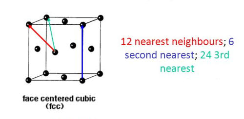
In the solid phase, the atoms (have been commanded, by the software, to) occupy an ordered FCC lattice structure, in which the atoms can only move by very small amounts as the structure vibrates – the atoms are essentially held still. Hence, there are far more peaks in the RDF corresponding to the long-range order in the crystalline structure. The first, second and third peaks in the RDF, at around r = 1.03, 1.49, and 1.83 correspond to the first, second and third nearest neighbours in the FCC lattice. The second nearest neighbour is the length of one side of the cubic unit cell, which was earlier calculated to be equal to 1.49380 (for a FCC lattice with a point number density of 1.2). The value of 1.49 from the RDF agrees well with the calculated value of 1.49380. In the FCC lattice, there are 12 nearest neighbours, 6 second nearest neighbours, and 24 third nearest neighbours, and the fact that the third peak in the RDF is of considerably greater intensity (g(r)) than the second reflects the fact that there are many more (4 times as many) second nearest neighbours in comparison to first nearest neighbours. The first, second and third nearest neighbours in the FCC lattice are illustrated in the diagram below:

It is worth noting that using the LJ cutoff of r = 3.2, neglecting interactions where r > 3.2, may have given rise to some error in the case of the liquid and gas simulations. It can be seen that the RDF of both the liquid and gas simulations have decayed to a constant value of g(r) = 1 when r > 3.2. In the case of the liquid simulation, it would not be surprising if a more accurate simulation with a higher LJ cutoff gave rise to further peak(s) in the RDF when r > 3.2, as well as better defined peaks that are closer to one another for r < 3.2. In the case of the gas simulation, using a higher LJ cutoff would likely result in a broader peak than that seen in the RDF above, that decays to the constant value of g(r) = 1 at a radius greater than 3.2.

TASK: In the D subfolder, there is a file liq.in that will run a simulation at specified density and temperature to calculate the mean squared displacement and velocity autocorrelation function of your system. Run one of these simulations for a vapour, liquid, and solid. You have also been given some simulated data from much larger systems (approximately one million atoms). You will need these files later.

Simulations were run for a vapour (density = 0.05), liquid (density = 0.8) and solid (density = 1.2, with lattice type set to fcc), at a reduced temperature of 1.0. The system contains 8000 atoms (20x20x20 grid).

TASK: make a plot for each of your simulations (solid, liquid, and gas), showing the mean squared displacement (the "total" MSD) as a function of timestep. Are these as you would expect? Estimate $D$ in each case. Be careful with the units! Repeat this procedure for the MSD data that you were given from the one million atom simulations.

The total MSD as a function of timestep for the solid, liquid and gas simulations carried out with N = 8000 and N = 1000000 have been plotted below, and a linear fit has been applied to each of these functions:

Each plot of the MSD vs time (timestep) is essentially a measure of how far particles in the system have moved with respect to time. In all cases we would expect the function to be linear, since any motion of particles in the system corresponds to random Brownian motion, rather than some external force acting on the particles. An upwards curve would indicate that there is some sort of drift of the molecules, due to some net force acting on the particles, and a plateau in the function would indicate that the particle is confined, or constrained, in some sort of way. In the case of the liquid, excellent linear behaviour is maintained throughout the simulation, however, in the solid and gas phases, it does require some time for linear behaviour to be established, and this could be attributed to the time required for the simulation to equilibrate following the initial random assignment of velocities to all of the particles. In the solid phase, oscillations can be seen that fade away, which can be thought of as anisotropic 'vibrations' in the system due to molecules in the ordered FCC lattice colliding backwards and forwards with one another over and over again, spreading the kinetic energy over the whole solid until equilibrium is reached, and the system does equilibrate relatively quickly. The MSD function for the gas phase, however, initially has an upwards curvature, indicating some sort of external force acting on the particles. The positive curvature in fact indicates that we are looking at the ballistic regime, which occurs in the gaseous phase since the density is so low that the atoms having a relatively long mean free path length. The gradient of the MSD for the gaseous calculations were only measured by considering the subsequent linear region into account, from around timestep 2250 onwards. This part of the function is known as the diffusive regime, and corresponds to the true random motion of particles in the system, and can therefore be used to calculate the diffusion coefficient of the system with adequate accuracy.

As expected, the gradient was greatest for the gas, followed by the liquid, whereas the gradient for the solid phase was essentially zero. This is because particles in the gas phase move the most (due to the lower density meaning movement of particles is not constricted by collisions), followed by those in the liquid. The fact that the solid function is essentially flat reflects the fact that the particles do not have net movement in the solid, but only some oscillations backwards and forwards at the beginning of the simulation as mentioned.

In the case of the liquid and gas simulations, increasing the size of the system from 8000 to 1000000 atoms doesn't seem to result in any great qualitative difference in terms of the MSD. However, in the case of the solid simulation it can clearly be seen that the MSD flattens out to a virtually straight line in the 1000000-atom simulation, whereas for the 8000-atom simulation, the function does not really completely flatten out over the course of the simulation, indicating that this smaller system size may not be quite large enough to gain accurate information in terms of the MSD. A larger-scale simulation of some system containing a greater number of particles will of course inherently result in better statistical information in each frame assessed compared to a smaller-scale simulation containing fewer particles.

The diffusion coefficient, D, was estimated by dividing the gradient of the linear fit by 6:

	Diffusion Coefficient / σ/√(ε/m*)
Phase	N = 8000	N = 1000000
Solid	8.3333 x 10-9	8.3333 x 10-10
Liquid	1.6667 x 10-4	1.6667 x 10-4
Gas	6.3333 x 10-3	6.0833 x 10-3

As expected, the diffusion coefficient is greatest for the gas and lowest for the liquid. The diffusion coefficient for the gas is just under one and a half orders of magnitude greater than that of the liquid, and roughly six orders of magnitude greater than that for the solid.

TASK: In the theoretical section at the beginning, the equation for the evolution of the position of a 1D harmonic oscillator as a function of time was given. Using this, evaluate the normalised velocity autocorrelation function for a 1D harmonic oscillator (it is analytic!):

$C\left(\tau \right)=\frac{\underset{-\mathrm{\infty }}{\overset{\mathrm{\infty }}{\int }}v\left(t\right)v(t+\tau )\mathrm{d}t}{\underset{-\mathrm{\infty }}{\overset{\mathrm{\infty }}{\int }}{v}^2\left(t\right)\mathrm{d}t}$

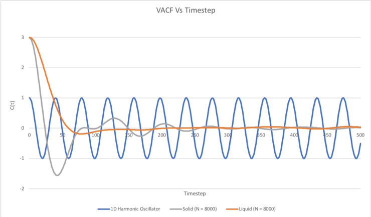
Be sure to show your working in your writeup. On the same graph, with x range 0 to 500, plot $C\left(\tau \right)$ with $\omega =1/2\pi$ and the VACFs from your liquid and solid simulations. What do the minima in the VACFs for the liquid and solid system represent? Discuss the origin of the differences between the liquid and solid VACFs. The harmonic oscillator VACF is very different to the Lennard Jones solid and liquid. Why is this? Attach a copy of your plot to your writeup.

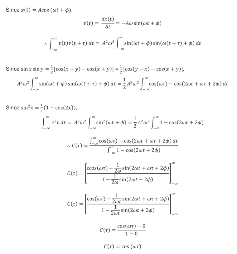
The normalised velocity autocorrelation function, C(τ), for a 1D harmonic oscillator was evaluated as follows:

C(τ) was plotted as a function of time (timestep (τ), between 0 and 500) for the 1D harmonic oscillator, as well as for the Lennard-Jones solid and liquid simulations carried out with N = 8000:

A minimum in a VACF corresponds to the velocities of the atoms in the system being negatively correlated (i.e. opposite) to their initial reference velocity, whereas a maximum corresponds to the velocities of the atoms in the system being positively correlated (i.e. similar) to their initial velocities (at timestep 0). When the VACF is equal to the that at the initial timestep (timestep = 0), e.g. when C(τ) = 1 in the case of the 1D harmonic oscillator, this basically means that the atoms are travelling at their initial velocities. For this reason, it makes sense that the VACF of the 1D harmonic oscillator oscillates between +1 and -1, reflecting the fact that the particles oscillate between some given maximum velocity, zero velocity, and the same given velocity in the opposite direction. No collisions occur in the 1D harmonic oscillator system that could destroy the correlation of the velocities of the particles with their initial velocities, hence the VACF doesn't decay to a constant value, C(τ) = 0.

In the case of the liquid and solid systems, the VACF quickly decays to a minimum, which can be thought of as occurring due to all particles in the system having collided. The minimum for the solid system is more pronounced than that for the liquid simulation because the atoms in the solid system form a more ordered FCC lattice, hence the particles will collide in a uniform fashion to give a clear, more definite negative correlation once all the particles in the system have collided. The minimum for the solid system also occurs more quickly (i.e. at an earlier timestep) in comparison to the liquid simulation, and this may be attributed to the greater density of the solid system resulting in more frequent collisions and therefore all of the particles having collided in a shorter timeframe. Also, a number of oscillations can be seen in the VACF of the Lennard-Jones solid, and this corresponds to the velocities of the atoms in the system fluctuating between being positively and negatively correlated to their initial velocities. This can essentially be thought of as the atoms in the system 'vibrating' as they collide back and forth between neighbouring atoms, since the structure is an ordered FCC lattice. This of course occurs until the kinetic energy has been dissipated evenly between all atoms in the solid, at which point the VACF has decayed to a constant value of 0.

TASK: Use the trapezium rule to approximate the integral under the velocity autocorrelation function for the solid, liquid, and gas, and use these values to estimate $D$ in each case. You should make a plot of the running integral in each case. Are they as you expect? Repeat this procedure for the VACF data that you were given from the one million atom simulations. What do you think is the largest source of error in your estimates of D from the VACF?

The trapezium rule was used to approximate the integral under the VACF, using a function that created trapezia of 1 timestep 'width'.

In all cases, the running integral converges to a constant value over the duration of the simulation, as expected. It takes considerably longer for this to occur in the gaseous simulation in comparison to that of the solid and liquid, for which the running integral converges quite quickly. This is due to the far lower density of the gas meaning the frequency of collisions in the system is much lower than that in the case of the solid and liquid simulations, therefore the time taken for the kinetic energy to be evenly distributed over all atoms in the system is far greater, thus the time taken for the VACF to decay to the constant value of 0 is considerably longer. Indeed, in the case of the gaseous simulation with N set to 1000000 atoms, the VACF had not fully decayed within the timeframe of the simulation, therefore the running integral had not completely converged. Hence, would be worthwhile to repeat this particular simulation for a slightly longer duration to gain more accurate information in terms of the diffusion coefficient.

D was calculated using the by dividing the integral of C(τ) over all τ (0 to 5000) by 3:

	Diffusion Coefficient / σ/√(ε/m*)
Phase	N = 8000	N = 1000000
Solid	0.060364158	0.022764742
Liquid	34.47327454	45.04573814
Gas	1089.389257	1634.232899

It can be seen that the diffusion coefficient (D) for the gas is just under 2 orders of magnitude greater than that of the liquid, and roughly four and a half orders of magnitude greater than that for the solid. This relative trend is what would be expected in terms of D for a solid, liquid and gas, and is somewhat similar to that calculated using the MSD, however the absolute values of D calculated using the VACFs are far greater than those calculated using the MSDs. Use of the trapezium rule (underestimates the area under maxima and overestimates the area under minima in a graph) when using the VACFs to calculate diffusion coefficients is an additional source of error that arises that is not a factor when using the MSD to calculate D, and could likely be the greatest source of error when estimating diffusion coefficients from the VACFs. Other sources of error in the estimations of D carried out could be use of the Lennard-Jones cutoff of 3σ, however this cutoff is quite standard when carrying out these kinds of simulations in research, and usually results in relatively accurate simulations of model systems in the literature. In addition, it is important that the Lennard-Jones model is indeed a good enough model for the system under investigation, otherwise the results obtained would not be appropriate. It is worth noting that these last two potential sources of error concerning the Lennard-Jones cutoff and appropriate use of the Lennard-Jones model itself is applicable to both calculations of D using the MSD and VACF methods.

References

- ↑ M. T. Ende, N. A. Peppas, J. Control. Release, 1997, 48, 47-56.
- ↑ 2.0 2.1 2.2 2.3 2.4 2.5 J. P. Hansen, L. Verlet, Phys. Rev., 1969, 184, 151.
- ↑ R. Huang, I. Chavez, K. M. Taute, B. Lukić, S. Jeney, M. G. Raizen and E.-L. Florin, Nat. Phys, 2011, 7, 576-580.
- ↑ 4.0 4.1 4.2 4.3 4.4 Y. Zhu, X. Lu, J. Zhou, Y. Wang and J. Shi, Fluid Ph. Equilibria, 2002, 194, 1141-1159.