Rep:Modxl9814

Theory

Velocity Verlet Algorithm

One way to solve Newton's Second law F=ma is the velocity-Verlet algorithm. By using a Taylor expansion,the atomic positions, velocities and accelerations can be approximated at time t with good precision. The position of atom i, at time t, is denoted by $x_i(t)$ and the velocity of the atom at time t is denoted by $v_i(t)$. Position at the next timestep $t+\delta t$ can be expressed by:

$x_i(t+\delta t)=x_i(t)+\frac{d{x}_i(t)}{dt}\delta t+\frac{1}{2!}\frac{d^2{x}_i(t)}{d{t}^2}\delta t^2+\frac{1}{3!}\frac{d^3{x}_i(t)}{d{t}^3}\delta t^3+O(\delta t^4)(1)$

A single timestep is expressed as:

$x(t+\delta t)=x_t+v_t\delta t+\frac{1}{2}{a}_t\delta t^2(2)$ $v(t+\delta t)=x_t+\frac{1}{2}(a_{t+\delta t}+a_t)\delta t(3)$

Fig 1: Classically calculated positions vs. velocity verlet calculated positions

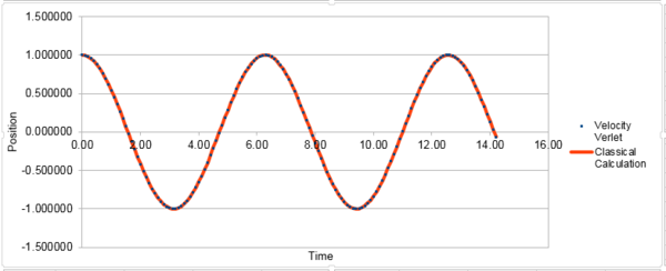
The classical harmonic oscillator can be describe by $x(t)=Acos(\omega t+\varphi )$. The errors oscillate through 5 peaks in the simulated time. The plot of the total energy vs. time of the simulated system:

Fig 2:Error vs. time

The cumulative error over a constant interval of time is given by:

$error(x(t_0+n\delta t))=O(\delta t^2)$

Thus, it can be seen from this equation that the relation between the maxima of the error of the Velocity-Verlet algorithm and $\delta t$ is quadratically increasing. The graph of the maxima of error vs. time therefore can be fit into the quadratic equation in figure 2.

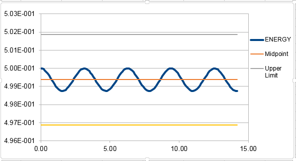
The total energy of the oscillating system is the sum of the kinetic energy and the potential energy, with $E_k=\frac{1}{2}m{v}^2$ and $E_p=\frac{1}{2}k{x}^2$. In this case, m=1 and k=1, therefore the equation is $E=\frac{v^2+x^2}{2}$.

Fig 3a:Energy vs. Time at 0.1 timestep with error limites of 0.5% on either side

Fig 3b:Energy vs. Time at 0.2 timestep with error limites of 0.5% on either side

In order for the total energy not to change by more than 1% over the course of the simulation, the timestep needs to be 0.2. It is important to monitor the total energy of the system to ensure that energy conservation is obeyed, the same as the real system.

Periodic Boundary Conditions

$1mL=1c{m}^3$. The density of water=$1g/c{m}^3$ under standard consitions (298K, 1atm). So the total mass of 1 mL water= 1g. The number of moles of water molecules=$\frac{1}{M_{H_{2}O}}=\frac{1g}{18g/mol}=0.056moles$

Therefore the total number of molecules in 1 mL of water=$n\times N_a=0.056\times 6.02\times 10^{23}=3.37\times 10^{22}$

The volume of 10,000 molecules of water=$\frac{10000}{3.37\times 10^{22}}=2.97\times 10^{-19}$

Equilibration

Creating the simulation box

Giving atoms random starting coordinates may make two atoms generated too close together. This will cause the two atoms to collide and arise the repulsion between the two atoms. The repulsive force between the atoms will drive them apart, leading to increase in the potential energy of the system and making it very unstable.

A face-centered cubic lattice has 4 lattice points per unit cell. The side length of the cubic unit cell=$\sqrt[3]{\frac{4}{1.2}}=1.49$

If 1000 unit cells were generated by the create_atoms command, 4000 atoms would be generated for a FCC lattice.

Setting the properties of the atoms

Mass 1 1.0

This means the mass of the single type of atom is 1.0.

Pair_style lj/cut 3.0

"Pair_style" indicates that the interaction is pairwise interaction. "lj.cut" describes the standard 12/6 Lennard-Jones potential without a Coulombic pairwise interaction. "3.0" indicates that the global cutoff for atoms is at 3.0.

Pair_coeff * *1.0 1.0

"pair_coeff" specifies the pairwise force field coefficients. The two asterisks indicate that the command will apply to all atoms.

If $x_i$ and $v_i$are specified,the Velocity-Verlet algorithm will be used for this simulation.

Running the simulation

The purpose of defining variable is that we don't need to manually change the numerical timestep each time the timestep needs to be changed. This reduces the human errors that may occur as the timestep only needs to be changed once to the value defined.

Checking equilibration

Fig 4a:Total energy vs. time at 0.001 timestep

Fig 4b: Temperature vs Time at 0.001 timestep

Fig 4c: Pressure vs. Time at 0.001 timestep

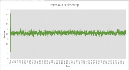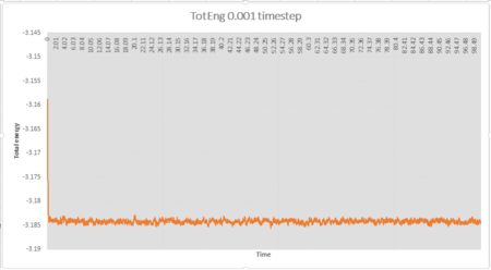
The simulation reaches equilibrium at 0.001 timestep as pressure and temperature become constant. It can be seen from pressure and temperature data that the simulation reaches equilibrium at t=0.29.The average pressure value is about 2.61 and the average temperature value is about 1.26.

Fig.5: Graph of energies for all timesteps

It can be seen from Fig 5 that the total energy produced by 0.0025 timestep are very close to those produced by 0.001 timestep. Simulations at 0.0075 and 0.01 also reach equilibrium but the total energies are higher than those produced by 0.001 timestep, thus these timesteps are not very accurate. Therefore the largest timestep to get acceptable results is 0.0025 and the worst choice is 0.015 timestep as the simulation doesn't reach equilibrium.

Running simulations under specific conditions

Examining the Input Script

The numbers 100 1000 100000 indicate the timesteps the input values will be used to compute the averages of density, pressure and temperature. For this simulation, the average will be calculated using values produced by timestep 100,200,...100000. Therefore, 1000 values will be used to calculate the average. The following line tells LAMMPS to run the simulation for 100000 timesteps. 0.0025 timestep will be used. Therefore 250 time units are simulated.

Plotting the Equations of State

Fig.6:Density vs Temperature and Ideal Gas law at p=2.3 and p=2.6

Fig.7:Density calculated by Ideal Gas Law compared to LJ model at P=2.3 and P=2.6

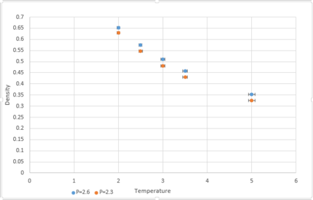
Simulations were conducted at temperatures 2,2.5,3,3.5,5 and pressures 2.3 and 2.6.

Heat Capacity Calculation

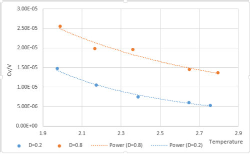
In the NVT ensemble, pressures (0.2,0.8) and temperatures (2,2.2,2.4,2.6,2.8) were used to calculate the heat capacity by using the following equation:

$C_V=\frac{\partial E}{\partial T}=\frac{\mathrm{V}\mathrm{a}\mathrm{r}\left[E\right]}{k_B{T}^2}=N^2\frac{⟨E^2⟩-{⟨E⟩}^2}{k_B{T}^2}$

The code to run the simulation in the NVT ensemble is as following:

variable density equal 0.2

### DEFINE SIMULATION BOX GEOMETRY ###
lattice sc ${density}
region box block 0 15 0 15 0 15
create_box 1 box
create_atoms 1 box

### DEFINE PHYSICAL PROPERTIES OF ATOMS ###
mass 1 1.0
pair_style lj/cut/opt 3.0
pair_coeff 1 1 1.0 1.0
neighbor 2.0 bin

### SPECIFY THE REQUIRED THERMODYNAMIC STATE ###
variable T equal 2.0
variable p equal 4
variable timestep equal 0.0025

### ASSIGN ATOMIC VELOCITIES ###
velocity all create ${T} 12345 dist gaussian rot yes mom yes

### SPECIFY ENSEMBLE ###
timestep ${timestep}
fix nve all nve

### THERMODYNAMIC OUTPUT CONTROL ###
thermo_style custom time etotal temp press
thermo 10

### RECORD TRAJECTORY ###
dump traj all custom 1000 output-1 id x y z

### SPECIFY TIMESTEP ###

### RUN SIMULATION TO MELT CRYSTAL ###
run 10000
unfix nve
reset_timestep 0

### BRING SYSTEM TO REQUIRED STATE ###
variable tdamp equal ${timestep}*100
variable pdamp equal ${timestep}*1000
fix nvt all nvt temp ${T} ${T} ${tdamp} 
run 10000
reset_timestep 0

### MEASURE SYSTEM STATE ###
thermo_style custom step etotal temp press atoms density vol
variable dens equal density
variable dens2 equal density*density
variable temp equal temp
variable volume equal vol
variable temp2 equal temp*temp
variable press equal press
variable press2 equal press*press
variable N2 equal atoms*atoms
variable E2 equal etotal*etotal
variable E equal etotal
fix aves all ave/time 100 1000 100000 v_dens v_temp v_press v_dens2 v_temp2 v_press2 v_E v_E2
unfix nvt
fix nve all nve
run 100000

variable avedens equal f_aves[1]
variable avetemp equal f_aves[2]
variable avepress equal f_aves[3]
variable errdens equal sqrt(f_aves[4]-f_aves[1]*f_aves[1])
variable errtemp equal sqrt(f_aves[5]-f_aves[2]*f_aves[2])
variable errpress equal sqrt(f_aves[6]-f_aves[3]*f_aves[3])
variable heatcapacity equal ${N2}*(f_aves[8]-f_aves[7]*f_aves[7])/f_aves[5]
variable CV equal ${heatcapacity}/${volume}

print "Averages"
print "--------"
print "Density: ${avedens}"
print "Stderr: ${errdens}"
print "Temperature: ${avetemp}"
print "Stderr: ${errtemp}"
print "Pressure: ${avepress}"
print "Stderr: ${errpress}"
print "heatcapacity: ${heatcapacity}"
print "volume: ${volume}"
print "heatcapacity/volume: ${CV}"

Fig.8: Cv/V vs. temperature at densities 0.2 and 0.8

Structural properties and the radial distribution function

Fig.9: g(r) vs. r for solid, liquid and gaseous phases

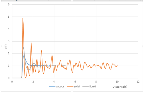
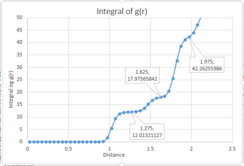
The radial distribution function was plotted for vapour, liquid and solid phases(Fig.9). The densities and temperatures were chosen from the phase diagram for the Lennard-Jones diagram.:

Phase	Density	Temperature
Vapour	0.1	1.2
Liquid	0.8	1.2
Solid	1.6	1.2

Fig.10: Integral of g(r) vs. interatomic distance for solid phase

Dynamical properties and the diffusion coefficient

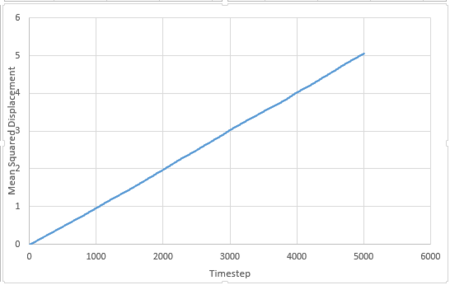
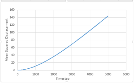
Mean Squared Displacement

The mean squared displacement is given by:

$\mathrm{M}\mathrm{S}\mathrm{D}\equiv ⟨(x-x_0{)}^2⟩=\frac{1}{N}\sum _{n=1}^N(x_n(t)-x_n(0){)}^2$

For 3375 atoms:

Fig 11a: Liquid simulation at d=0.8, T=1.2

Fig 11b: Gas simulation at d=0.1, T=1.2

Fig 11c: Solid simulation at d=1.6, T=1.2

For 1 million atoms:

Fig 12a: Liquid simulation at d=0.8, T=1.2

Fig 12b: Gas simulation at d=0.1, T=1.2

Fig 12c: Solid simulation at d=1.6, T=1.2

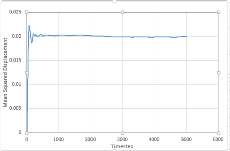The diffusion coefficient is given by:

$D=\frac{1}{6}\frac{\delta ⟨r^2⟩}{\delta t}$

$\delta ⟨r^2⟩$ is the slope of the trendline of the mean squared displacement vs. timestep plot. The timestep $\delta t=0.002$.

Velocity Autocorrelation Function

The equation of the position of a 1D harmonic oscillator is:

$x(t)=A\cos (\omega t+\varphi )$

$v(t)=\frac{dx}{dt}$, thus:

$v(t)=\frac{d(Acos(\omega t+\varphi )}{dt}=-A\omega sin(\omega t+\varphi )$

and

$v(t+\tau )=-A\omega sin(\omega (t+\tau )+\varphi )$

Therefore, by substitution:

$C(\tau )=\frac{\underset{-\mathrm{\infty }}{\overset{\mathrm{\infty }}{\int }}v(t)v(t+\tau )\mathrm{d}t}{\underset{-\mathrm{\infty }}{\overset{\mathrm{\infty }}{\int }}{v}^2(t)\mathrm{d}t}=\frac{\underset{-\mathrm{\infty }}{\overset{\mathrm{\infty }}{\int }}-A\omega sin(\omega t+\varphi )\times -A\omega sin(\omega (t+\tau )+\varphi )\mathrm{d}t}{\underset{-\mathrm{\infty }}{\overset{\mathrm{\infty }}{\int }}(-A\omega sin(\omega t+\varphi ){)}^2\mathrm{d}t}=\frac{(A\omega {)}^2\underset{-\mathrm{\infty }}{\overset{\mathrm{\infty }}{\int }}sin(\omega t+\varphi )sin(\omega (t+\tau )+\varphi )\mathrm{d}t}{(A\omega {)}^2\underset{-\mathrm{\infty }}{\overset{\mathrm{\infty }}{\int }}si{n}^2(\omega t+\varphi )\mathrm{d}t}=\frac{\underset{-\mathrm{\infty }}{\overset{\mathrm{\infty }}{\int }}sin(\omega t+\varphi )sin(\omega (t+\tau )+\varphi )\mathrm{d}t}{\underset{-\mathrm{\infty }}{\overset{\mathrm{\infty }}{\int }}si{n}^2(\omega t+\varphi )\mathrm{d}t}$

Since $sin(x+y)=sin(x)cos(y)+cos(x)sin(y)$:

$C(\tau )=\frac{\underset{-\mathrm{\infty }}{\overset{\mathrm{\infty }}{\int }}sin(\omega t+\varphi )[sin(\omega t+\varphi )cos(\omega \tau )+cos(\omega t+\varphi )sin(\omega \tau )]\mathrm{d}t}{\underset{-\mathrm{\infty }}{\overset{\mathrm{\infty }}{\int }}si{n}^2(\omega t+\varphi )\mathrm{d}t}=\frac{cos(\omega \tau )\underset{-\mathrm{\infty }}{\overset{\mathrm{\infty }}{\int }}si{n}^2(\omega t+\varphi )\mathrm{d}t}{\underset{-\mathrm{\infty }}{\overset{\mathrm{\infty }}{\int }}si{n}^2(\omega t+\varphi )\mathrm{d}t}+\frac{sin(\omega \tau )\underset{-\mathrm{\infty }}{\overset{\mathrm{\infty }}{\int }}sin(\omega t+\varphi )cos(\omega t+\varphi )\mathrm{d}t}{\underset{-\mathrm{\infty }}{\overset{\mathrm{\infty }}{\int }}si{n}^2(\omega t+\varphi )\mathrm{d}t}=cos(\omega \tau )+\frac{sin(\omega \tau )\underset{-\mathrm{\infty }}{\overset{\mathrm{\infty }}{\int }}sin(\omega t+\varphi )cos(\omega t+\varphi )\mathrm{d}t}{\underset{-\mathrm{\infty }}{\overset{\mathrm{\infty }}{\int }}si{n}^2(\omega t+\varphi )\mathrm{d}t}$

Since $sin(2x)=2sin(x)cos(x)$:

$C(\tau )=cos(\omega \tau )+\frac{sin(\omega \tau )\underset{-\mathrm{\infty }}{\overset{\mathrm{\infty }}{\int }}\frac{1}{2}sin(2(\omega t+\varphi ))\mathrm{d}t}{\underset{-\mathrm{\infty }}{\overset{\mathrm{\infty }}{\int }}si{n}^2(\omega t+\varphi )\mathrm{d}t}$

As $sin(x)$ is an odd function, the area above the x-axis and below the x-axis cancel out from negative infinity to positive infinity. Thus, $\underset{-\mathrm{\infty }}{\overset{\mathrm{\infty }}{\int }}sin(2(\omega t+\varphi ))=0$. therefore:

$C(\tau )=cos(\omega \tau )$

Fig.14: VACF for solid, liquid and 1D Harmonic Oscillator

The minima in the VACF for the liquid system represent the collisions between the atoms and the solvent molecules and change in direction. The minima in the VACF for the solid system represent the collisions between the atoms and change in direction. The minima for the solid system is lower than the minima for the liquid system because of the stronger interatomic forces. The VACF for the liquid system only has one weak oscillation, this is because the atoms only interact with their closest neighbor. In the VACF for the solid system, there are more oscillations as the atoms can vibrate in fixed positions. The harmonic oscillator VACF is very different to the Lennard Jones liquid and solid as there are no interactions between the atoms so the atoms will always vibrate with constant velocity without loss in energy. Therefore, the amplitude doe not change.

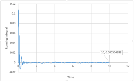
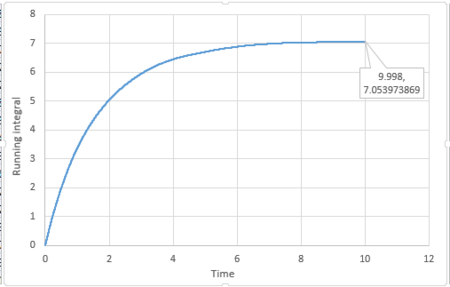
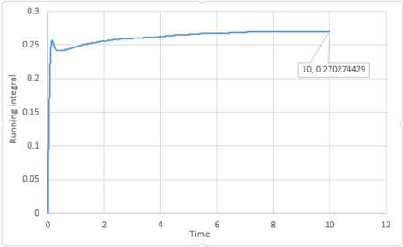
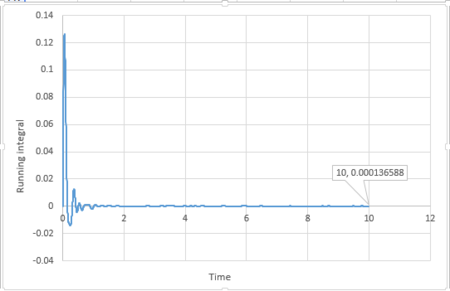
By applying the trapezium rule, integral under VACF can be calculated and running integral can be plotted:

For 3375 atoms:

Fig.15a: running integral vs. time for liquid

Fig.15b: running integral vs. time for solid

Fig.15c: running integral vs. time for gas

For 1 million atoms:

Fig.16a: running integral vs. time for liquid

Fig.16b: running integral vs. time for solid

Fig.16c: running integral vs. time for gas

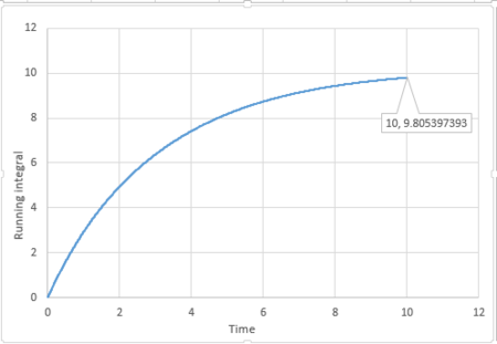The diffusion coefficient is calculated by:

$D=\frac{1}{3}\underset{0}{\overset{\mathrm{\infty }}{\int }}\mathrm{d}\tau ⟨\mathbf{v}\left(0\right)\cdot \mathbf{v}\left(\tau \right)⟩$

The last point of the running integral is $\underset{0}{\overset{\mathrm{\infty }}{\int }}\mathrm{d}\tau ⟨\mathbf{v}\left(0\right)\cdot \mathbf{v}\left(\tau \right)⟩$.

For 3375 atoms: Liquid: $D=\frac{1}{3}\times 0.2937=9.79\times 10^{-2}$; Solid: $D=\frac{1}{3}\times 5.64\times 10^{-4}=1.88\times 10-4$; Gas: $D=\frac{1}{3}\times 7.054=2.351$;

For 1 million atoms: Liquid: $D=\frac{1}{3}\times 0.2703=9.01\times 10^{-2}$; Solid: $D=\frac{1}{3}\times 1.37\times 10^{-4}=4.57\times 10^{-5}$; Gas: $D=\frac{1}{3}\times 9.805=3.268$.

The diffusion coefficient calculated from this method was largest for gas, followed by liquid and then gas. The coefficients for the larger system were very similar to the ones for the smaller system. The coefficients calculated by MSD were similar to the ones calculated by VACF for liquid and gas, but the coefficient calculated by VACF was larger than the one calculated by MSD for solid. The largest source of error may be that the trapezium rule overestimates the area under the solid curve as the timestep is not small enough.