
Rep:Module 3 - ceg09
This project aims to demonstrate the power of computational chemistry in predicting the optimal structures of not only reagents and products but also those of transition states. Transition state modelling is very important as it is often extremely hard to analyze transition states experimentally and it allows us to obtain clear information about the nature of a reaction pathway.
A range of computational methods will be used throughout and their differences highlighted as part of this report.
Cope Rearrangement
Introduction

The cope rearrangement is a [3,3]-sigmatropic shift reaction first developed by Arther Cope in the 1940's[1]. In this section we will explore such a reaction between two 1,5-hexadiene molecules using computational methods. The reaction involves the concerted breaking of 2 bonds and formation of a new σ-bond, passing through either a so-called "chair" or "boat" transition state. Studies have shown[2] the "boat" structure to be higher in energy at the B3LYP/6-31G* level of theory. Similar computational methods will be employed here hoping to align with the results from previous studies.
Optimization of Reactants & Products
First of all, the minimal energy conformations were found using the Hartree-Fock method with a 3-21G basis set . The results are shown below:
| Structure | Corresponding Appendix Structure | Image | Energy (Hartrees) | Relative Energy (kcal/mol) | Point Group |
|---|---|---|---|---|---|
| Gauche 1 - visualize | Gauche 4 |  |
-231.69153 | 0.71 | C2 |
| Gauche 2 - visualize | Gauche 2 |  |
-231.69167 | 0.62 | C2 |
| Gauche 3[3] - visualize | Gauche 3 |  |
-231.69266 | 0.00 | C1 |
| Gauche 4 - visualize | Gauche 1 |  |
-231.68772 | 3.10 | C2 |
| Gauche 5 - visualize | Gauche 6 |  |
-231.68962 | 2.20 | C1 |
| Gauche 6 - visualize | Gauche 5 |  |
-231.68962 | 1.91 | C1 |
| Anti 1 - visualize | As appendix |  |
-231.69260 | 0.04 | C2 |
| Anti 2 - visualize |  |
-231.69254 | 0.08 | Ci | |
| Anti 3[4] - visualize |  |
-231.68907 | 2.25 | C2h | |
| Anti 4[5] - visualize |  |
-231.69097 | 1.06 | C1 |
It can be seen that the most stable structure is gauche 3 followed by anti 1 and anti 2 respectively. These three minimized structures were then further optimized using a higher level DFT B3LYP method and basis set 6-31G(d).
| Structure | Energy (Hartrees) | Relative Energy (kcal/mol) | Point Group |
|---|---|---|---|
| Gauche 3[6] - visualize | -234.61133 | 0.29 | C1 |
| Anti 1[7] - visualize | -234.61179 | 0.00 | C2 |
| Anti 2[8] - visualize | -234.61171 | 0.05 | Ci |
After further optimization, the geometries remain extremely similar however the energy values and relative order of the three conformers has changed. The change in the energy values themselves is simply a consequence of using a different optimization method. Whilst values calculated using the same method can be compared, it is not possible to compare numerical values between two calculation methods. However, the relative energies can be compared and yield interesting results.
Under the B3LYP/6-31G* level of theory the anti 1 conformer is seen to be lowest in energy compared to the HF/3-21G level which calculates the gauche 3 conformer to be the most stable. This discrepancy is most likely due to the differences in accuracy between the two methods. The DFT (B3LYP) method builds upon the HF method, combining it with an additional calculated exchange energy and so is much more accurate. In addition, the 3-21G basis set is of low accuracy especially when compared to the more advanced 6-31G* set. All in all it is fair to say that the B3LYP/6-31G* method is much more accurate and indeed often aligns well with corresponding experimental results.


The relative energies found under the B3LYP method can be explained by considering the intramolecular interactions involved in stabilizing the anti and gauche conformers. It is known that[9] interactions between σ and σ*-orbitals lead to a stabilizing effect as shown in the diagram to the right. These interactions are maximal when the σ and σ*-orbitals are in an anti-periplanar (app) configuration, that is, with a dihedral angle of 180°. The table below summarizes such interactions for both the gauche 3 and anti 1 conformer.
| Gauche 3 | Anti 1 | |||
|---|---|---|---|---|
 |

| |||
| Stabilizing Orbital Interaction | Dihedral Angle(s) (°) | Stabilizing Orbital Interaction | Dihedral Angle(s) (°) | |
| 2 x σC-C/σ*C-H | 171 and 173 | 4 x σC-H/σ*C-H | 178 and 178 | |
| 2 x σC-H/σ*C-C | ||||
| 2 x σC-H/σ*C-H | 179 | 2 x σC-C/σ*C-C | 177 | |
As you can see the anti 1 σ/σ* interactions are all very close to perfectly app configurations whereas the gauche 3 conformer has two angles that are slightly lower than this optimal 180° angle. This slight deviation from the optimal app geometry means that the stabilization from the σC-C/σ*C-H and σC-H/σ*C-C interactions will be lessened. In addition, the energy profile for these types of interactions, shown above, shows that the E2/stabilization energy is maximized when the σ-σ* energy gap is reduced. This can be achieved when you have a good σ-donor (high in energy) and a good σ*-acceptor (low in energy). All in all, the anti 1 conformer has the best combination of donor-acceptor orbitals and so will have the largest total E2 value and hence be the most stable.
| It is known that a second stabilizing effect of van der Waals dispersion forces between two non-bonded atoms can in fact favour the gauche conformation. This is a longer ranging effect often seen between hydrogens at non-bonding distances and is maximal at the sum of the van der Waals radii for the two interacting atoms, 2.4Å for H...H interaction (this type of interaction will be discussed further in later sections). Closer examination of this effect could be carried out with the gauche conformer expected to have more favourable contacts than the anti conformer. |
Frequency Analysis
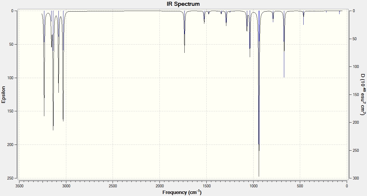
Frequency analysis works by taking the 2nd derivative of the potential energy surface of the system. If all of the frequencies generated by the frequency analysis are positive the optimized geometry or minimum on the potential energy surface has been found, however if one of the frequency values is negative a maximum point/transition state has been found. All of the frequencies calculated for all 3 conformers were positive and the C=C vibrations are shown below.
| Structure | Frequency (cm-1) | Intensity | Description | Image/Animation |
|---|---|---|---|---|
| Anti 1[10] - Click here to visualize IR spectrum | 1732 | 4.73 | Symmetric C=C stretch | 
|
| 1735 | 13.55 | Asymmetric C=C stretch | 
| |
| Anti 2[11] - Click here to visualize IR spectrum | 1731 | 0.00 | Symmetric C=C stretch | 
|
| 1734 | 18.1 | Asymmetric C=C stretch | 
| |
| Gauche 3[12] - Click here to visualize IR spectrum | 1731.86 | 6.89 | Symmetric C=C stretch | 
|
| 1733 | 6.13 | Asymmetric C=C stretch | 
|
Energies
Computational frequency analysis is not only a powerful tool for accurately predicting infra-red vibration frequencies but also for providing key energetic data from the system. Thermochemical data from the frequency analysis provides us with 4 key pieces of information:
- Sum of electronic and zero point energies - the sum of the system's potential energy at 0K and the system's zero-point vibrational energy (Eelec + ZPE)
- Sum of electronic and thermal Energies - the energy of the system under standard conditions, 298.15K and 1 atm. This includes the vibrational, translational and rotational energies also under standard conditions (E + Evib + Erot +Etrans)
- Sum of electronic and thermal Enthalpies - the energy including an enthalpic RT correction
- Sum of electronic and thermal Free Energies - the entropic contribution to the free energy
The results for standard conditions along with the results from frequency analysis conducted at 0K (in fact, 0.00001K) are shown below:
| Anti 1[13] | Anti 2[14] | Gauche 3[15] |
|---|---|---|
| At 293.15K | ||
Sum of electronic and zero-point Energies= -234.469298 Sum of electronic and thermal Energies= -234.461966 Sum of electronic and thermal Enthalpies= -234.461022 Sum of electronic and thermal Free Energies= -234.500862 |
Sum of electronic and zero-point Energies= -234.469204 Sum of electronic and thermal Energies= -234.461857 Sum of electronic and thermal Enthalpies= -234.460913 Sum of electronic and thermal Free Energies= -234.500777 |
Sum of electronic and zero-point Energies= -234.468693 Sum of electronic and thermal Energies= -234.461464 Sum of electronic and thermal Enthalpies= -234.460520 Sum of electronic and thermal Free Energies= -234.500105 |
| At 0K | ||
Sum of electronic and zero-point Energies= -234.468861 Sum of electronic and thermal Energies= -234.468861 Sum of electronic and thermal Enthalpies= -234.468861 Sum of electronic and thermal Free Energies= -234.468861 |
Sum of electronic and zero-point Energies= -234.468766 Sum of electronic and thermal Energies= -234.468766 Sum of electronic and thermal Enthalpies= -234.468766 Sum of electronic and thermal Free Energies= -234.468766 |
Sum of electronic and zero-point Energies= -234.468256 Sum of electronic and thermal Energies= -234.468256 Sum of electronic and thermal Enthalpies= -234.468256 Sum of electronic and thermal Free Energies= -234.468256 |
As you can see at 0K/absolute zero there is no thermal contribution, as is the definition of absolute zero, and all of the energies are equal to the sum of electronic and zero-point energy.
This type of frequency analysis can be conducted under many difference conditions of temperature, pressure etc. Further study of the effects of varying the temperature and pressure would prove interesting. On raising the temperature one would expect the following results:
|
Optimization of Chair & Boat Transition States
So far we have demonstrated the use of computational chemistry in determining optimal structures, vibrational data and energetic information for individual reactant systems. Another perhaps more useful computational technique is the modelling and analysis of transition states. Transition states are extremely hard to isolate/observe experimentally as they correspond to a maximum on the system's potential energy surface hence are very unstable. For this reason it is clearly very useful to be able to model such structures in order to gain valuable information about the reaction pathway, perhaps helping to improve and better understand synthetic methods.
The possible boat and chair transition structures of the hexadiene cope rearrangement will be optimized and analyzed in order to explain the relative stability of the chair structure as discussed in section 1.1.
Chair
Optimization


In order to generate the optimized chair transition state, an initial allyl fragment was first optimized using the HF/3-21G method, the structure of which can been seen on the right. Two of these fragments were then combined and optimized in 2 different fashions which are explained in detail below. The initial "guessed" structure is displayed to the right.
| Method Number | 3D Visualization | Method | Terminal C-C Bond Distance (Å) | ||
|---|---|---|---|---|---|
| C14-C6 | C9-C1 | ||||
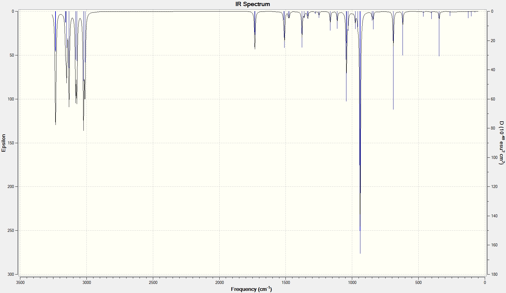
| 1 | Type = Optimization and frequency Optimization to = TS (Berny) Resulting imaginary frequency = -817.9cm<sup>-1</sup> Additional parameters = Force constants calculated once |
2.02 | 2.02 | ||
| 2 | a | Type = Optimization Optimization to = Minimum Additional parameters = redundant coordinates use to freeze the terminal C-C distances to 2.2Å |
2.20 | 2.20 | |
| b | Type = Optimization and frequency Optimization to = TS (Berny) Additional parameters = Optimized structure from part a taken and redundant coordinates use to set the derivative of the terminal C-C distances. Force constants never calculated |
2.02 | 2.02 | ||
 |
The presence of a negative/imaginary vibration shows that a transition state has been found, to see the IR spectrum click here. This imaginary frequency directly relates to the Cope rearrangement effectively showing the breaking and the formation of bonds.It is clear that whilst two different methods were used to optimize the chair transition structure they both yield the same terminal C-C bond lengths and so can be said to be reliable methods.
|
Intrinsic Reaction Coordinate
Another useful computational tool is the calculation of the intrinsic reaction coordinate (IRC). The IRC takes the previously found transition state structure and follows the minimum reaction pathway along the system's reaction coordinate until a local minimum is found. This is very useful when trying to predict the most likely product moving away from the transition state.
In this case, the reaction pathway is symmetrical and so the IRCs will only be calculated in the forwards direction. Several different parameters were tested to find which set of conditions gave the most accurate results.
| Number of Points Along IRC | Calculate Force Constants | IRC Animation | IRC Data |
|---|---|---|---|
| 50[16] | once |  |

|

| |||
| 100[17] | once |  |

|

| |||
| 50[18] | always |  |

|

|
The structure of the molecule at the end of the IRC is the minimum energy structure moving away from the transition state and so in theory should be the reaction product. This final structure was optimized using HF/3-21G[19], the results of which are shown below:
| Final IRC Structure | Energy (Hartrees) | Gauche 2 Structure | Energy (Hartrees) | |
|---|---|---|---|---|
 |
-231.69167 | c.f. | |
-231.69167 |
As you can see the energy of the final IRC structure is identical to the energy of the Gauche 2 conformer found in section 1.2.
Boat
Optimization


In order to optimize the boat transition state the QST2 method will be used. Unlike the demonstrated methods for the chair optimization, in which a "guessed" transition state structure must be used, the QST2 method takes the reactants and products and finds a transition state between them. It is noted that the atomic labels of the reactants and products must be identical for this method to work.
Initially, the optimized anti 2 structure was used as the basis for the reactant and product structures, shown to the right. When the QST2 transition state was optimized[20] straight from this structure the job failed. This is because the QST2 method only linearly interpolates between the reactant and product and does not rotate any of the bonds. In effect it only translates the structures. In order to overcome this problem, the central C9-C1-C4-C7 dihedral was set to 0° and the two internal C9-C1-C4 and C7-C4-C1 angles set to 100°.
Unfortunately, the structure (click here to visualize) calculated by this method was seen to be asymmetric and so suggested that the true minimal chair transition state structure had not been found. Observation of the frequency log file[21] shows that two imaginary/negative frequencies were calculated showing that neither a minimum nor a maximum point on the potential energy surface was found. These imaginary frequencies are shown below:
 Low frequencies --- -681.9496 -339.2038  -66.2980  -60.6073  -36.1093    0.0002
 Low frequencies ---    0.0007    0.0008  208.6869
This problem arises when no force constants are calculated as the computational process effectively guesses a value that can sometimes be wrong. The optimization was carried out for a second time specifying to calculate the force constants once and indeed a successful optimization structure was obtained (click here to visualize).
| Image | Terminal C-C Bond Length Å | Imaginary Frequency (cm-1)- click here to visualize IR spectrum | Motion of Imaginary Frequency |
|---|---|---|---|
 |
2.14 | -839.92 | 
|
The terminal C-C bond length is seen to be attractive, this is discussed further in section 5.2.
Intrinsic Reaction Coordinate
The same IRC analysis was conducted for the boat transition structure however the force constants were always calculated in both cases.
| Number of Points Along IRC | Calculate Force Constants | IRC Animation | IRC Data | Final Structures |
|---|---|---|---|---|
| 50 | always |  |
 |

|

| ||||
| 100 | always |  |
 |

|

|
The final IRC structure was again optimized using HF/3-21G[23] and seen to be equivalent to the gauche 3 conformer.
| Final IRC Structure | Energy (Hartrees) | Gauche 3 Structure | Energy (Hartrees) | |
|---|---|---|---|---|
 |
-231.69266 | c.f. | |
-231.69266 |
Overall Activation Energies
Shown below are the calculated activation energies of the cope rearrangement via both the chair and boat transition states. The results reflect the reported relative stabilities of the two transition states where the boat structure, under both levels of theory, was found to have a higher activation energy and be less stable than the chair structure.
| HF/3-21G | B3LYP/6-31G* | Literature Activation Energy (kcal/mol) | |||||||
|---|---|---|---|---|---|---|---|---|---|
| Structure | Energy (Hartrees) | Corresponding Hexadiene Conformer Energy (Hartrees) | Activation Energy (Hartrees) | Activation Energy (kcal/mol) | Energy (Hartrees) | Corresponding Hexadiene Conformer Energy (Hartrees) | Activation Energy (Hartrees) | Activation Energy (kcal/mol) | |
| Gauche 3 | Anti 1 | ||||||||
| Chair | -231.61932 | -231.69266 | 0.07334 | 46.0 | -234.55698 | -234.61179 | 0.05481 | 34.4 | 33.5±0.5 |
| Boat | -231.60280 | -231.69266 | 0.08986 | 56.4 | -234.54309 | -234.61179 | 0.0687 | 43.1 | 44.7±2.0 |
As you can see the B3LYP/6-31G* method yielded results that were very similar to the experimental values whereas the values calculated under the HF/3-21G method were not so comparable. This is most likely due to the lower accuracy of both the HF method and 3-21G basis set as discussed previously.
Conclusion
This section has demonstrated the power of computational chemistry to quantitatively explain observed experimental and theoretical trends. The differences between two methods of differing levels of theory have been highlighted showing the B3LYP/6-31G* method to be consistently more accurate. In addition, IRC analysis has allowed us to model the relaxation of the transition state into products and also to identify the products' structures.
Clearly a great deal of valuable information can be obtained via computational techniques. The methods used in this section will now be further applied to more complex systems.
Diels-Alder Cycloaddition - Butadiene + Ethene

The Diels-Alder reaction is an example of a [4s+2s] cycloaddition and is a very important synthetic tool. It also provides an interesting system for computational analysis.
First of all a relatively simple system of butadiene and ethene will be examined.
Reactant Optimization
Both butadiene and ethene were optimized first using the semi-empirical AM1 method then using the DFT B3LYT/6-31G* method. The results of which along with the HOMO and LUMO molecular orbitals (MOs) are displayed below. It is noted that, in terms of MO symmetry, s refers to a symmetric orbital with respect to the plane and a to an asymmetric orbital.
| Molecule | AM1 | B3LYP/6-31G* | ||||||||
|---|---|---|---|---|---|---|---|---|---|---|
| Energy (Hartrees) | RMS | MOs | MO Symmetry | Energy (Hartrees) | RMS | MOs | MO Symmetry | |||
| Butadiene | 0.48797 | 0.0000175 | HOMO |  |
a | -155.98595 | 0.0000567 | HOMO |  |
a |
| LUMO |  |
s | LUMO |  |
s | |||||
| Ethene | 0.02619 | 0.0000252 | HOMO |  |
s | -78.58746 | 0.0001445 | HOMO |  |
s |
| LUMO |  |
a | LUMO |  |
a | |||||
You can that there is no visible difference between the MOs generated using AM1 and DFT which is encouraging. This, however, is not always the case. Here we are dealing with a relatively simple system hence the continuity of the results. For more complex the systems we will see later, this agreement is not always so clear and should be expected when using two different computational methods.
In addition, it is clear that the LUMO of ethene and the HOMO of butadiene both have the same symmetry hence there is a favorable overlap between the two leading to a "reaction".
Transition State Optimization
Following the optimization of the reactants, their optimized structures were then aligned once again in a guessed transition state geometry in order to optimize to the transition state. The fragments were aligned so that the two forming σ-bonds were approximately 2Å. The system was optimized to a TS(Berny) with the force constants calculated once, the results are shown below:
| AM1 | B3LYP/6-31G* | Frequency Analysis | ||||||||
|---|---|---|---|---|---|---|---|---|---|---|
| Energy (Hartrees) | RMS | MOs | MO Symmetry | Energy (Hartrees) | RMS | MOs | MO Symmetry | |||
| 0.11165 | 0.00002973 | HOMO |  |
a | -234.54389655 | 0.00000826 | HOMO |  |
s | Both of the methods showed one imaginary frequency at -956.42 and -524.81 for AM1 and B3LYP respectively
(animation does not always run, please click to visualize) It is noted that the imaginary frequency corresponds to the synchronous formation of the two new σ-bonds in the product |
| LUMO |  |
s | LUMO |  |
s | |||||

| MO of the Transition State | Reactant MO Combination: | |
|---|---|---|
| Butadiene | Ethene | |
| LUMO | LUMO | HOMO |
| HOMO (AM1) | HOMO | LUMO |
At first HOMOs generated by the two different computational methods appear to be different. Further analysis of the MOs shows that in fact several sets of degenerate orbitals were found and in all of the examined cases these degenerate pairs simply flipped moving between the two different methods. This is perhaps more clearly demonstrated visually below. The three sets of degenerate orbitals are highlighted in yellow in the energy diagram.
| Relative MO Energy Levels | Method | HOMO-5 | HOMO-4 | HOMO-3 | HOMO-2 | HOMO-1 | HOMO | LUMO |
 |
AM1 |  |
 |
 |
 |
 |
|
|
| DFT |  |
 |
 |
 |
 |
|
|
This discrepancy is due to the different ways in which each method calculated MOs and in their differing accuracies. The B3LYP/6-31G* method is much more accurate hence it would be reasonable to assume that its results are more reliable. Having said this, from the data shown above the DFT HOMO can be said to be a combination of the butadiene LUMO and ethene HOMO. This combination of reactant orbitals has already been used to form the transition state LUMO and hence would not in fact be available.
| Further MO analysis would need to be conducted in order to explained the aforementioned discrepancy in LCAO analysis. |

Another interesting approach to analyzing transition state structures is to consider the distance between the atoms forming new bonds in the product. In 1924 John Lennard-Jones first proposed a potential energy surface showing the interaction between two atoms/nuclei[24]. This model still holds true and can be used to explain how molecular orbitals overlap resulting in a stabilizing effect. A simple Lennard-Jones potential is displayed to the right and shows that, most simply, there are 4 key regions on the potential energy curve:
- Repulsive region - at very small internuclear distances the nuclei are so close together that they repel one another and the energy tends towards infinity.
- Equilibrium bond distance - this is the minimum on the potential energy curve where the most stable interaction is found. This is equal the length of the bond between two atoms at equilibrium.
- Dissociation limit - this is the region in which the two atoms are too far apart to interact and are essentially two separate atoms.
Finally, there is the 4th region in which the atoms move closer and closer until finally a bond is formed. This is the region in which attractive van der Waals interactions stabilize the system and may eventually lead to bond formation. It is the region in which the transition state structure is found. Van der Waals interactions are observed between atoms that are separated by a distance equal to the sum of their van der Waals radii. This is because it is at this distance that the electron densities/MOs of each atom begin to overlap. The van der Waals radius for a carbon atom it approximately 1.6Å and so attractive interactions will be felt when the C-C internuclear distance is <3.2Å. These terminal C-C contacts for the transition state are shown below along with other C-C bond lengths.
| Method | Ethene C=C | Diene C=Cs | Diene C-C | Terminal C-C distance/bond being formed |
|---|---|---|---|---|
| AM1- visualize | 1.38 | 1.38 | 1.40 | 2.12 |
| B3LYP/6-31G* - visualize | 1.39 | 1.38 | 1.41 | 2.27 |
As you can see the terminal C-C distance is considerably lower than 3.2Å proving that a new σ-bond is indeed being formed in the transition state. The C-C bonds are also all very similar in length i.e. there are no longer distinct C-C single and C=C double bonds. This again fits with a delocalized transition state structure in which bonds are being broken and formed.
| Intrinsic reaction coordinate analysis was not conducted here however could be used to examine the product of the reaction. |
Diels-Alder Cycloaddition - Hexadiene + Maleic Anhydride

A more complex Diels-Alder reaction will now be examined, that of cyclohexa-1,3-diene and maleic anhydride. An interesting characteristic of many Diels-Alder reactions is the selectivity between endo- and exo-products. The kinetically formed endo-product is often favoured[25] and can be explained by considering the molecular orbitals involved in the formation of the transition state. MO analysis will be conducted here in order to support this observation. It is also important to note that the exo-transition state/product has a higer torsional strain due to the more compressed dihedral angles, as discussed in module 1[26].
Reactant Optimization
Once again the reactants were optimized using both AM1 and B3LYP/6-31G* methods. The results are shown below:
| Molecule | AM1 | B3LYP/6-31G* | ||||||||
|---|---|---|---|---|---|---|---|---|---|---|
| Energy (Hartrees) | RMS | MOs | MO Symmetry | Energy (Hartrees) | RMS | MOs | MO Symmetry | |||
| Cyclohexadiene | -0.02771[27] | 0.000005 | HOMO |  |
a | -233.419[28] | 0.000032 | HOMO |  |
a |
| LUMO |  |
s | LUMO |  |
s | |||||
| Maleic Anhydride | -0.12182[29] | 0.000037 | HOMO |  |
s | -379.2895[30] | 0.000141 | HOMO |  |
a |
| LUMO |  |
a | LUMO |  |
a | |||||
The HOMO and LUMOs show the correct symmetry for favourable interactions with the exception of the maleic anhydride HOMO calculated using the B3LYP method. This was again found to be due to a "flipping" of degenerate MOs between the two methods however the results have not been shown in order to make this report of a reasonable size!
Transition State Optimization
The optimized reactants were then combined and the frozen coordinates method, explained in section 3.1, used to set the distance between the two sets of carbon atoms forming new bonds to 2Å.
| Transition State Structure | AM1 Optimization Results | B3LYP/6-31G* Optimization Results | Frequency Analysis | ||||||
| Energy (Hartrees) | RMS | MOs | Energy (Hartrees) | RMS | MOs | ||||
| Exo | -0.050420 | 0.000020 | HOMO |  |
-612.67931095[31] | 0.00001137 | HOMO |  |
A single imaginary frequency was found at -812.15cm-1 and 448.22cm-1for AM1 and B3LYP/6-31G* respectively, proving that a transition state structure was found.
|
| LUMO |  |
LUMO | 
| ||||||
| Endo | -0.051504[32] | 0.000006 | HOMO |  |
-612.68339677[33] | 0.00000460 | HOMO |  |
A single imaginary frequency was found at -806.36cm-1 and -447.03cm-1 for AM1 and B3LYP/6-31G* respectively, proving that a transition state structure was found.
|
| LUMO |  |
LUMO | 
| ||||||


Once again some variation is seen between the two methods however the MOs are all relatively similar. The optimization results clearly support the relatively stabilization of the endo-transition state with the endo- being 0.0011 Hartrees lower in energy than the exo.
Further MO Analysis
The endo-selectivity commonly observed for Diels-Alder reactions can be explained by secondary orbital overlap. Shown below are the LUMO+1 and LUMO+2 for both the endo- and exo-transition states. It can be seen that whilst their is a clear favourable interaction between the -(C=O)-O-(C=O)- fragment and the cyclohexadiene orbitals in the endo-structure, in the exo-structure a nodal plane is observed. This missing secondary orbital overlap stabilization in the exo-transition state explains why the endo-structure is more stable and hence favoured.
| Endo | Exo | |
|---|---|---|
| LUMO+2 |  |

|
| LUMO+1 |  |

|
Intrinsic Reaction Coordinate

IRC analysis was conducted for both the endo- and exo-transition states, the results of which are shown below. A simple energy profile, shown to the right, shows that the system is asymmetric and so the IRC must be initially calculated in both the forwards and reverse directions. It is clear from the IRC energy profiles as well as the final forwards and backwards structures that for the exo-transition state the IRC runs backwards in order to form products and the endo- forwards. It can also be seen that IRC when run away from the products takes the transition state back to the reactants as is expected.
| Structure | Number of Points Along IRC | Calculate Force Constants | IRC Animation | IRC Data | Final Structures | |
|---|---|---|---|---|---|---|
| Forwards | Backwards | |||||
| Endo | 10[34] | Once |  |
 |
 |

|

| ||||||
| Exo | 50 | Once |  |
 |
 |

|

| ||||||

Interestingly, both of the final "products" look very similar hence further IRC analysis and optimization was used to examine the true nature of these structures.
The product formed via the kinetic/endo-pathway is expected to be higher in energy than the thermodynamic/exo-product. However, the IRC produced two identical products with the same energies suggesting that both transition states lead to the same product. A revised reaction profile has been drawn, shown to the right, however further analysis of the products using a higher level of theory is needed to distinguish between the two structures and to draw a more definite picture of the overall reaction pathway.
| Structure | IRC Data[35] | Energy of Final Optimized Structure (Hartrees) | Image of Final Structure |
|---|---|---|---|
| Endo - |  |
0.16[36] | 
|

| |||
| Exo - |  |
0.16[37] | 
|

|
Conclusion
Once again computational analysis has successfully predicted the optimal structures of reactants, products and transition states. The so-called "endo-rule" has been shown by examining the relative energies of endo- and exo-transition states. Some interesting results concerning endo- and exo-products have been obtained and would perhaps provide a good basis for further computational exploration.
References
- ↑ DOI:10.1021/ja01859a055
- ↑ DOI:10.1021/ja00101a078
- ↑ http://hdl.handle.net/10042/to-12471
- ↑ http://hdl.handle.net/10042/to-12473
- ↑ http://hdl.handle.net/10042/to-12474
- ↑ http://hdl.handle.net/10042/to-12475
- ↑ http://hdl.handle.net/10042/to-12476
- ↑ http://hdl.handle.net/10042/to-12477
- ↑ http://www.ch.ic.ac.uk/local/organic/conf/
- ↑ http://hdl.handle.net/10042/to-12478
- ↑ http://hdl.handle.net/10042/to-12479
- ↑ http://hdl.handle.net/10042/to-12480
- ↑ Frequency Analysis at 0K - http://hdl.handle.net/10042/to-12482
- ↑ Frequency Analysis at 0K - http://hdl.handle.net/10042/to-12483
- ↑ Frequency Analysis at 0K - http://hdl.handle.net/10042/to-12481
- ↑ http://hdl.handle.net/10042/to-12487
- ↑ http://hdl.handle.net/10042/to-12489
- ↑ http://hdl.handle.net/10042/to-12488
- ↑ http://hdl.handle.net/10042/to-12493
- ↑ http://hdl.handle.net/10042/to-12484
- ↑ http://hdl.handle.net/10042/to-12485
- ↑ http://hdl.handle.net/10042/to-12486
- ↑ http://hdl.handle.net/10042/to-12492
- ↑ DOI:10.1098/rspa.1924.0082
- ↑ DOI:10.1002/1521-3773(20020517)41:10
- ↑ https://wiki.ch.ic.ac.uk/wiki/index.php?title=Module_1_-_ceg09#Dimerisation
- ↑ http://hdl.handle.net/10042/to-12508
- ↑ http://hdl.handle.net/10042/to-12507
- ↑ http://hdl.handle.net/10042/to-12509
- ↑ http://hdl.handle.net/10042/to-12510
- ↑ http://hdl.handle.net/10042/to-12499
- ↑ http://hdl.handle.net/10042/to-12503
- ↑ http://hdl.handle.net/10042/to-12498
- ↑ http://hdl.handle.net/10042/to-12502
- ↑ Endo - http://hdl.handle.net/10042/to-12500 & Exo - http://hdl.handle.net/10042/to-12501
- ↑ http://hdl.handle.net/10042/to-12497
- ↑ http://hdl.handle.net/10042/to-12496