Rep:Module 2 - ceg09

This module will explore the power of computational analysis in the field of inorganic chemistry. Bonding in inorganic systems is often much more complex than organic molecules and so computational techniques provide an invaluable tool for characterizing inorganic bonding and structures. Computational studies will be used here to examine molecular orbitals, natural bond orbitals and characteristic infra red frequencies as well as to find energetically optimized structures.

Optimization is the iterative process of finding the lowest energy configuration/the global minimum on the system's potential energy surface. This is done by solving the Schrödinger first for the electron density, assuming fixed nucleus position, and then for nuclear positions. The DFT B3LYP method of optimization will be used throughout due to its speed however this does mean comprising on the accuracy of the results. A range of basis sets will be used and explained in further detail when necessary.

Please note that all of the jobs submitted to the HPC server have been published and the links displayed in the final section of this report for your reference.

BH₃

Optimization

The optimized geometry of a trigonal planar BH₃ molecule was first found using the B3LYP (DFT) method with basis set 3-21G, a very low accuracy basis set however it does provide fast calculation times. First of all it is important to check that the optimization converged i.e. was able to find the energy minimum/stationary point:

Item               Value     Threshold  Converged?
 Maximum Force            0.000413     0.000450     YES
 RMS     Force            0.000271     0.000300     YES
 Maximum Displacement     0.001610     0.001800     YES
 RMS     Displacement     0.001054     0.001200     YES
 Predicted change in Energy=-1.071764D-06
 Optimization completed.
    -- Stationary point found.

Now we are happy that we have achieved the optimal geometry we can proceed to examine the rest of the results in more detail.The results below show that all 3 equilibrium B-H bond lengths are 1.19Å and all dihedral angles are 120° as is expected for D_3h geometry, click here to visualize the BH₃ molecule in 3D. The bond lengths are in extremely good agreement with the literature value of 1.19Å^[1].

                           ----------------------------
                           !   Optimized Parameters   !
                           ! (Angstroms and Degrees)  !
 --------------------------                            --------------------------
 ! Name  Definition              Value          Derivative Info.                !
 --------------------------------------------------------------------------------
 ! R1    R(1,2)                  1.1935         -DE/DX =    0.0004              !
 ! R2    R(1,3)                  1.1935         -DE/DX =    0.0004              !
 ! R3    R(1,4)                  1.1935         -DE/DX =    0.0004              !
 ! A1    A(2,1,3)              120.0            -DE/DX =    0.0                 !
 ! A2    A(2,1,4)              120.0            -DE/DX =    0.0                 !
 ! A3    A(3,1,4)              120.0            -DE/DX =    0.0                 !
 ! D1    D(2,1,4,3)            180.0            -DE/DX =    0.0                 !
 --------------------------------------------------------------------------------

The results summary below supports the highly symmetrical D_3h geometry for the BH₃ molecule, reporting a dipole moment of 0 Debye. The reported root mean squared (RMS) gradient norm value of 0.0002 Hartrees/Bohr also supports the accuracy of the calculations. The closer to 0 Hartrees/Bohr the value of RMS the more accurate the data as we are looking to find an energy minimum/stationary point where RMS=0 Hartrees/Bohr.

BH3Optimisation
File Name = BH3
File Type = .log
Calculation Type = FOPT
Calculation Method = RB3LYP
Basis Set = 3-21G
Charge = 0
Spin = Singlet
E(RB3LYP) = -26.46226338 a.u.
RMS Gradient Norm = 0.00020672 a.u.
Imaginary Freq =
Dipole Moment = 0.0000 Debye
Point Group = D3H
Job cpu time:  0 days  0 hours  0 minutes

The graphical representations of the optimization process, displayed to the right, show that it took a total of 4 iterations to obtain the energy minimum of -26.46 hartrees at which the RMS gradient norm reached 0.00 hartree/bohr.

Frequency

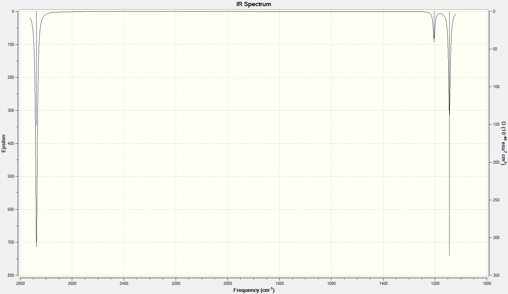
After having optimized the geometry of the BH₃ molecule, frequency analysis was used to examine its vibrational modes. This analysis generates an IR spectrum and allows us to further proved that we have indeed found the global minimum, equilibrium geometry, and not a transition state structure. Frequency analysis works by taking the 2^nd derivative of the potential energy surface of the system. If all of the frequencies generated by the frequency analysis are positive the optimized geometry/ global minimum has been found, however if one of the frequency values is negative a maximum point/transition state on the potential energy surface has been found.

BH3Freq2
File Name = CEG09_BH3_FREQ
File Type = .log
Calculation Type = FREQ
Calculation Method = RB3LYP
Basis Set = 3-21G
Charge = 0
Spin = Singlet
E(RB3LYP) = -26.46226442 a.u.
RMS Gradient Norm = 0.00004830 a.u.
Imaginary Freq = 0
Dipole Moment = 0.0001 Debye
Point Group = C2V
Job cpu time:  0 days  0 hours  0 minutes 13.0 seconds.

The data below shows the "low frequencies" from the vibrational analysis. The top line are the 6 so-called "zero" frequencies and correspond to motions of the system's centre of mass and so should be close to zero and certainly much lower than the 1st "real" frequency, shown on the 2^nd line. The low accuracy of the basis set used to generate these results explains why the "zero" frequencies are perhaps a little higher than we would ideally like however the highest "zero" frequency, 40.5cm^-1, is indeed an order of magnitude lower then the lowest "real" frequency, 1146.1cm^-1, and therefore the results can be said to be reliable.

Low frequencies ---   -0.0007    0.0005    0.0006   35.6548   39.6598   40.4759
 Low frequencies --- 1146.0881 1204.8810 1204.9797

IR Frequencies For Optimized BH₃ - Click here to visualize the IR spectrum
Frequency (cm^-1)	Literature^[2] (cm^-1)	Difference (%)	Intensity	Description	Symmetry
1146	1148	0.2	92.7	The concerted, symmetric bending of all 3 B-Br bonds	a₂"
1205	1197	0.7	12.4	The concerted bending of 2 B-Br bonds	e'
1205	1197	0.7	12.4	The wag-type movement, bending of 1 Tl-Br bond	e'
2592	2503	3.6	0.0	The totally symmetric mode in which all 3 B-H bonds stretch and compress in a concerted manor	a₁'
2730	2602	4.9	103.9	The asymmetric stretching of 2 B-Br bonds	e'
2730	2602	4.9	103.8	The symmetric stretching of 2 B-Br bonds together with the relatively asymmetric stretching of the remaining B-Br bond	e'

As you can see all of the generated frequencies are positive proving that the global minimum has been found. In addition, they are all well within the relatively large error range for vibrational frequencies and are in fact, relatively speaking, extremely accurate compared to the literature.

It is noted that although there are 3N-6, 6 for BH₃ , possible vibrational modes, there are only 3 signals in the IR spectrum. This is because the ?????? signal to 2591.61 cm^-1 is totally symmetrical hence has no change in dipole and so is not observed in the spectrum. In addition, the modes found at 1204.88 and 1204.98 as well as 2729.89 and 2730.15 are both symmetrically degenerate pairs and so form 2 single peaks.

MO

Simple LCAO is often a very useful tool in predicting the shapes of molecular orbitals, especially for small molecules. Unfortunately for larger systems this method can become extremely complicated hence why computational analysis is often used in conjunction with, or as an alternative to, the LCAO method. Here the power of computational methods for generating MOs will be demonstrated using BH₃ and compared to the more straightforward LCAO approach.

It is clear that whilst the computational MOs are more sophisticated they are in fact very similar to those predicted by LCAO. In addition, computational analysis has also allowed us to quantitatively predict the relative order of the doubly degenerate 2e' MOs and the 3a₁' MO. This is not so easy to do using the LCAO method alone. Clearly computational analysis is a powerful tool for molecular analysis, both in terms of its accuracy and in its ability to quantify the MO energies. It is noted that the 1a₁' orbital is much lower in energy than the other MOs, at -6.7 Hartrees, as shown by the relative MO energies diagram to the left however has be included in the overall MO diagram for completion.

NBO

The data below shows the charge distribution over the BH₃ system. Boron is the more electropositive atom and so as expected is seem to carry less electron density than the hydrogen atoms.

Summary of Natural Population Analysis:                 
                                                         
                                       Natural Population
                Natural  -----------------------------------------------
    Atom  No    Charge         Core      Valence    Rydberg      Total
 -----------------------------------------------------------------------
      B    1    0.33161      1.99903     2.66935    0.00000     4.66839
      H    2   -0.11054      0.00000     1.11021    0.00032     1.11054
      H    3   -0.11054      0.00000     1.11021    0.00032     1.11054
      H    4   -0.11054      0.00000     1.11021    0.00032     1.11054
 =======================================================================
   * Total *    0.00000      1.99903     6.00000    0.00097     8.00000

The data below describes the orbital characteristics of each bond i.e. the hybridization. It is clear that for the first 3 bonds, the boron atom contributes approximately 44% of the electron density in the bond (expected due to lower electronegativity); a 1/3 of which is s-character and 2/3 p-character corresponding to 3 sp² hybridized orbitals as is expected for the optimized BH3 structure with dihedral angles of 120°. The remaining 56% of the electron density comes from the 3 respective H atoms all of which are 100% s-character. This supports the expected B-H σ-sigma bonding between an s-orbital on H and an sp² orbital on B. The 4th orbital is the core boron s-orbital and the 5th orbital the empty (denoted by LP*) p-orbital on boron. The calculations describe this 5th orbital as being 100% s-character however we know that this is not the case. This discrepancy is most likely due to the low accuracy of the basis set used and general computational error.

(Occupancy)   Bond orbital/ Coefficients/ Hybrids
 ---------------------------------------------------------------------------------
     1. (1.99853) BD ( 1) B   1 - H   2 
                ( 44.48%)   0.6669* B   1 s( 33.33%)p 2.00( 66.67%)
                                            0.0000  0.5774  0.0000  0.0000  0.0000
                                            0.8165  0.0000  0.0000  0.0000
                ( 55.52%)   0.7451* H   2 s(100.00%)
                                            1.0000  0.0000
     2. (1.99853) BD ( 1) B   1 - H   3 
                ( 44.48%)   0.6669* B   1 s( 33.33%)p 2.00( 66.67%)
                                            0.0000  0.5774  0.0000  0.7071  0.0000
                                           -0.4082  0.0000  0.0000  0.0000
                ( 55.52%)   0.7451* H   3 s(100.00%)
                                            1.0000  0.0000
     3. (1.99853) BD ( 1) B   1 - H   4 
                ( 44.48%)   0.6669* B   1 s( 33.33%)p 2.00( 66.67%)
                                            0.0000  0.5774  0.0000 -0.7071  0.0000
                                           -0.4082  0.0000  0.0000  0.0000
                ( 55.52%)   0.7451* H   4 s(100.00%)
                                            1.0000  0.0000
     4. (1.99903) CR ( 1) B   1           s(100.00%)
                                            1.0000  0.0000  0.0000  0.0000  0.0000
                                            0.0000  0.0000  0.0000  0.0000
     5. (0.00000) LP*( 1) B   1           s(100.00%)

TlBr₃

Optimisation

For the optimization of TLBr₃ the DFT B2LYP method was used along with a LanL2DZ basis set. The LanL2DZ basis set is a pseudo-potential in which the core electrons are essentially "frozen" in order to simplify the calculations.

 Item               Value     Threshold  Converged?
 Maximum Force            0.000002     0.000450     YES
 RMS     Force            0.000001     0.000300     YES
 Maximum Displacement     0.000022     0.001800     YES
 RMS     Displacement     0.000014     0.001200     YES
 Predicted change in Energy=-6.083939D-11
 Optimization completed.
    -- Stationary point found.

Bond angles of 120° and bond lengths of 2.65Å were observed and are in good agreement with the literature^[3] value of 2.52Å.

                           ----------------------------
                           !   Optimized Parameters   !
                           ! (Angstroms and Degrees)  !
 --------------------------                            --------------------------
 ! Name  Definition              Value          Derivative Info.                !
 --------------------------------------------------------------------------------
 ! R1    R(1,2)                  2.651          -DE/DX =    0.0                 !
 ! R2    R(1,3)                  2.651          -DE/DX =    0.0                 !
 ! R3    R(1,4)                  2.651          -DE/DX =    0.0                 !
 ! A1    A(2,1,3)              120.0            -DE/DX =    0.0                 !
 ! A2    A(2,1,4)              120.0            -DE/DX =    0.0                 !
 ! A3    A(3,1,4)              120.0            -DE/DX =    0.0                 !
 ! D1    D(2,1,4,3)            180.0            -DE/DX =    0.0                 !
 --------------------------------------------------------------------------------

As with the BBr₃ analysis the data below supports the validity of the calculations. The optimization process can been seen to converge after 3 cycles reaching an RMS value extremely close to zero.

TlBr3Optiimisation
File Name = TlBr3_Optimisation
File Type = .log
Calculation Type = FOPT
Calculation Method = RB3LYP
Basis Set = LANL2DZ
Charge = 0
Spin = Singlet
E(RB3LYP) = -91.21812851 a.u.
RMS Gradient Norm = 0.00000090 a.u.
Imaginary Freq =
Dipole Moment = 0.0000 Debye
Point Group = D3H
Job cpu time:  0 days  0 hours  0 minutes 30.0 seconds.

Frequency

The same method, DFT B3LYP, and basisi set, LanL2DZ, as used for the optimization was used for the frequency analysis. The "zero" frequencies are all seen to be close to zero and well below the lowest "real" frequency. In addition the first real frequency is positive proving that the global minimum was found and not a transition state.

Low frequencies --- -3.4214 -0.0026 -0.0004 0.0015 3.9361 3.9361 Low frequencies --- 46.4289 46.4292 52.1449	1 E' Frequencies -- 46.4289 Red. masses -- 88.4613 Frc consts -- 0.1124 IR Inten -- 3.6867

IR Frequencies For Optimized TlBr₃: click here to visualize the IR spectrum
Frequency (cm^-1)	Intensity	Description	Symmetry
46	3.7	The concerted bending of 2 of the Tl-Br bonds	e'
46	3.7	The wag-type movement, bending of 1 Tl-Br bond	e'
52.	5.8	The symmetric bending of all 3 Tl-Br Bonds	a₂"
165	0.0	The concerted, symmetric stretching of all 3 Tl-Br bonds	a₁'
211	25.5	The asymmetric stretching of 2 Tl-Br bonds	e'
211	25.5	The symmetric stretching of 2 Tl-Br bonds together with an asymmetric stretch of the remaining Tl-Br bond	e'

As seen for BBr₃, not all vibrations results in an observable peak in the IR spectrum. The 2 vibrations at 46cm^-1 and the two at 211cm^-1 are both degenerate pairs and so coalesce into 2 single peaks. The vibration at 165cm^-1 is totally symmetrical with no change in dipole moment hence no observable IR peak.

Mo(CO)₄(PCl₃)₂ Isomers

The study of cis- and trans-complexes are often used in undergraduate study to explain and explore the nature of infra red spectrometry. Indeed as an undergraduate at Imperial a 2^nd year inorganic laboratory experiment dealt with the cis- and trans-isomers of Pt(PPh₃)₂(CO)₂ and their corresponding IR spectra. A similar exploration will be conducted here using Pt(Cl)₂(CO)₂. PPh₃ ligands are not used here as they require very complex calculations, Cl is a good substitute as it occupies a similar spacial volume however is much easier to handle.

Optimization

The two isomers were first optimized using the B3LYP (DFT) method with LanL2MB basis sets. The optimization was also set to "loose" in order to aid convergence. After this initial optimization the structures were manually altered so as to ensure that the global minimum, rather than a local minimum, is found. The cis-isomer was manipulated to give a C-Pt-P-Cl dihedral angle of 180° and the trans-isomer to align on of the Cl atoms parallel to one of the C=O groups.

Next, using the same B3LYP method, a pseudo-potential basis set LanL2DZ was applied and the manually edited structures optimized. The results of this final optimization are displayed below.

Cis2ndOptimisation
File Name = Cis2ndOptimisationOutput
File Type = .log
Calculation Type = FOPT
Calculation Method = RB3LYP
Basis Set = LANL2DZ
Charge = 0
Spin = Singlet
E(RB3LYP) = -623.57707194 a.u.
RMS Gradient Norm = 0.00000671 a.u.
Imaginary Freq =
Dipole Moment = 1.3096 Debye
Point Group = C1
Job cpu time:  0 days  1 hours  8 minutes  9.2 seconds.

 Trans2ndOptimisation
File Name = Trans2ndOptimisationOutput
File Type = .log
Calculation Type = FOPT
Calculation Method = RB3LYP
Basis Set = LANL2DZ
Charge = 0
Spin = Singlet
E(RB3LYP) = -623.57603102 a.u.
RMS Gradient Norm = 0.00003170 a.u.
Imaginary Freq =
Dipole Moment = 0.3052 Debye
Point Group = C1
Job cpu time:  0 days  0 hours 47 minutes  5.6 seconds.

        Item               Value     Threshold  Converged?
 Maximum Force            0.000026     0.000450     YES
 RMS     Force            0.000006     0.000300     YES
 Maximum Displacement     0.001286     0.001800     YES
 RMS     Displacement     0.000323     0.001200     YES
 Predicted change in Energy=-1.222187D-08
 Optimization completed.
    -- Stationary point found.

         Item               Value     Threshold  Converged?
 Maximum Force            0.000067     0.000450     YES
 RMS     Force            0.000020     0.000300     YES
 Maximum Displacement     0.001049     0.001800     YES
 RMS     Displacement     0.000179     0.001200     YES
 Predicted change in Energy=-7.952286D-08
 Optimization completed.
    -- Stationary point found.

As you can see, according to these results the cis-isomer is approximately 0.001 Hartrees lower in energy than the trans-isomer. It is reported in the literature^[4] however that the corresponding PPh₃ trans-isomer is the most stable with the cis-isomer in fact readily converting to the trans-form at room temperature. The observed energy difference falls well within the error range of approximately 0.0038 Hartrees and so is most likely a simple error in the calculations rather than a case of the thoroughly examined and reported norm being wrong.

Bond Lengths For Optimized Cis-Mo(CO)₄(PCl₃)₂ - Click here to visualize the molecule in 3D		Bond Lengths For Optimized Trans-Mo(CO)₄(PCl₃)₂ - Click here to visualize the molecule in 3D
Bond Type	Bond Length (Å)	Bond Type	Bond Length (Å)
Mo-C	2.01	Mo-C	2.06
Mo-P	2.51	Mo-P	2.44
C-O	1.17	C-O	1.17
P-Cl	2.24	P-Cl	2.24

Frequency

IR Frequencies For Optimized Cis-Mo(CO)₄(PCl₃)₂ - Click here to visualize the IR spectrum
Frequency (cm^-1)	Intensity	Description
11	0	Symmetric, rocking movement about the Mo-P bond
18	0	Asymmetric, rocking movement about the Mo-P bond
1945	763	The asymmetric stretching of the cis-pair (trans to PCl₃) of CO groups
1949	1499	The asymmetric stretching of the axial/trans pair of CO groups
1958	633	The concerted, symmetric stretching of both CO pairs (opposite to one another). Asymmetric stretching relative to one another.
2023	598	The concerted, symmetric stretching of all 4 CO groups.

IR Frequencies For Optimized Trans-Mo(CO)₄(PCl₃)₂ - Click here to visualize the IR spectrum
Frequency (cm^-1)	Intensity	Description
5	0	Symmetric, rocking movement about the Mo-P bond
6	0	Asymmetric, rocking movement about the Mo-P bond
1950	1475	The asymmetric stretching of one of the trans-pairs of CO groups
1951	1467	The asymmetric stretching of the other trans-pairs of CO groups
1977	1	The concerted, symmetric stretching of both CO pairs (opposite to one another). Asymmetric stretching relative to one another.
2031	4	The concerted, symmetric stretching of all 4 CO groups.

Comparison of the CO regions in the IR spectra for the cis- and trans-isomer clearly shows 2 distinct peaks for the cis- and only 1 for the trans-isomer. As can be seen from the data table above for the trans-isomer the peaks at 1977 and 2031^cm-1 have a very low intensity. This is due to the highly symmetrical D_4h geometry of the trans-isomer. The aforementioned stretches do not result in a change in dipole and therefore are not observed in the IR spectrum. The corresponding stretches for the cis-isomer, with C2v symmetry, on the other hand does give a change in dipole and hence is observed in the spectrum. In addition all of the CO peaks observed in both the cis- and trans-spectra are double degenerate hence why only 1 peak is seen for 2 "different" stretches.

Comparison of CO Region In the IR Spectra for Cis- and Trans-Mo(CO)₄(PCl₃)₂
Cis-isomer	Trans-isomer

What Is a Bond?

As seen in the first part of this module Gaussian often neglects to draw bonds that we know do in fact exist. This happens because Gaussian works upon a predetermined set of inter-atomic when drawing bonds (or not). If the inter-atomic distances are longer than those specified in Gaussian's database then no bond will be drawn. In addition, many of the predetermined bonding distances are based upon organic systems. It is well known that inorganic systems can exhibit much larger bonding distances however are often determined by Gaussian to be non- bonding.

Perhaps the most concise way to describe a bond is the stabilizing interaction between the electronic systemsof the atoms involved. This can be electrostatic (ionic bonding) or a favorable overlap of electron density (covalent).

Mini Project

Introduction

Over the last few years, the interest in boron containing compounds' use as high temperature semiconductors, superconductors and possibly high energy fuels has grown. In particular there have been several studies into so-called bare B₆ clusters, that us to say B₆ clusters containing no H atoms.

There have been many varied suggestions for the lowest energy conformation of these B₆ clusters. In this section the optimized geometry of 3 such configurations will be examined along with their molecular orbitals and NBO. A 2003 report^[5] by Jun Ma, Zhenhua Li, Kangnian Fan and Mingfei Zhou conducted similar analysis and so in this section the focus will be to compare their results to my own. Other approaches may have been followed including a comparison of LanL2DZ and B3lYP/6-31+G(d) methods however a literary comparison seemed to be more valuable.

It is noted that whenever the "literature" cited, this is in reference to the report by J. Ma et al.^[6].

Optimization

Each molecule was optimized within GaussView 5.0 using the B3LYP/6-31+G(d) (DFT) method. It is noted that the additional structure 4, shown to the right, was initially investigated however the frequency analysis showed that the optimized structure was not an energy minimum and therefore will not be examined further. The results for structure 4 have however been included in the D-Space publications for reference.

The literature reports that fully planar form of structure 1 is the most stable structure, 1.4kcal/mol lower in energy (using B3LYP/6-311+G(3df))than structure 2. It is important to note here that the reported literature values fall into the approximate ±10kj/mol (2.4kcal/mol) error range and so it is quite possible that the two structures were in fact in the opposite relative energetic ordering, i.e. 2 more stable than 1. It is also noted that structure we shall refer to as 1 is in fact a bent form relative to structure 1 in the literature. The planar form was not found to be an energy minimum whereas the bent version was.

It was observed during this project that structure 2 is approximately 8.2kcal/mol lower in energy than structure 1. The energy difference calculated in this project between structures 1 and 2, approximately 34kj/mol, falls outside the error range and so, with a great deal of caution, could be seen to be more reliable than the data in the literature and would suggest that structure 2 is in fact the more stable. Further analysis of the planar form of structure 1, along with the 5 reported isomers not analyzed here, would be required to support this argument.

In order to better align with the literature and so conduct a more realistic comparison, the optimization for structures 1 and 2 were also conducted using the B3LYP/6-311+G(3df) method. This however yielded similar results and so only continued to contradict the literature.

Structure 3 was found to be overall the highest in energy, approximately 2300kj/mol higher in energy than structure 2.

Optimisation Data for the 3 B₆ Isomers
1	2	3


Item Value Threshold Converged? Maximum Force 0.000012 0.000450 YES RMS Force 0.000006 0.000300 YES Maximum Displacement 0.000553 0.001800 YES RMS Displacement 0.000274 0.001200 YES Predicted change in Energy=-2.425428D-08 Optimization completed. -- Stationary point found.	Item Value Threshold Converged? Maximum Force 0.000273 0.000450 YES RMS Force 0.000129 0.000300 YES Maximum Displacement 0.001475 0.001800 YES RMS Displacement 0.000597 0.001200 YES Predicted change in Energy=-1.633203D-06 Optimization completed. -- Stationary point found.	Item Value Threshold Converged? Maximum Force 0.000002 0.000450 YES RMS Force 0.000001 0.000300 YES Maximum Displacement 0.000019 0.001800 YES RMS Displacement 0.000007 0.001200 YES Predicted change in Energy=-2.124677D-10 Optimization completed. -- Stationary point found.
Structure1_bent_Opt File Name = Bent_Opt_Output File Type = .log Calculation Type = FOPT Calculation Method = RB3LYP Basis Set = 6-31+G(d) Charge = 0 Spin = Singlet E(RB3LYP) = -148.79214084 a.u. RMS Gradient Norm = 0.00000974 a.u. Imaginary Freq = Dipole Moment = 1.6256 Debye Point Group = C1 Job cpu time: 0 days 0 hours 13 minutes 45.8 seconds.	Structure_2_Optimization_631G File Name = 631G_Output File Type = .log Calculation Type = FOPT Calculation Method = RB3LYP Basis Set = 6-31+G(d) Charge = 0 Spin = Singlet E(RB3LYP) = -148.80545884 a.u. RMS Gradient Norm = 0.00026077 a.u. Imaginary Freq = Dipole Moment = 3.1472 Debye Point Group = C5V Job cpu time: 0 days 0 hours 1 minutes 13.3 seconds.	Structure_4_Optimisation_621G File Name = 631G_Output File Type = .log Calculation Type = FOPT Calculation Method = RB3LYP Basis Set = 6-31+G(d) Charge = 0 Spin = Singlet E(RB3LYP) = -148.71378080 a.u. RMS Gradient Norm = 0.00000273 a.u. Imaginary Freq = Dipole Moment = 0.0000 Debye Point Group = D4H Job cpu time: 0 days 0 hours 1 minutes 31.8 seconds.

The bond lengths have not been tabulated however can be visualized on the 3D molecules (links above). For structures 2 and 3, for which there is a direct literature comparison, the bond lengths were extremely similar to those in the literature. Structure 1, although bent relative to the literature, also showed very similar bond lengths and a similar B1-B5-B3 bond angle.

Molecular Orbital (MO) Analysis

MO analysis of the three B₆ structures is shown below and shows some interesting results. It is noted that the MO generated for structure 3 correlate very well with the literature.

MOs for The Three B₆ Isomers
	LUMO+1	LUMO	HOMO	HOMO-1	HOMO-2	HOMO-3	HOMO-4	HOMO-5	HOMO-6
1
2
3

The MOs for structure 1 have been examined in more depth below.It it noted that some of the orbitals that are described as being delocalised may not at first appear as such however this is simply due to the settings chosen when capturing the MO images. unfortunately time constraints did not allow for this to be rectified.

Further MO Analysis of Structure 1
Orbital	Description	Orbital	Description
LUMO+1		HOMO-3	A delocalised л-system formed by the 6 p-orbitals pointing above and below the plane.
LUMO	A delocalised л-system formed by the 6 p-orbitals pointing above and below the plane.	HOMO-4	Delocalised σ-orbitals
HOMO	3c-2e bond with 2 p-orbitals pointing into the centre of the system.	HOMO-5	An anti-bonding MO
HOMO-1	Delocalised σ-orbitals	HOMO-6	A delocalised л-system formed by the 6 p-orbitals pointing above and below the plane.
HOMO-2	An anti-bonding MO

There are several discrepancies between the data obtained in this project and the literature report. The MOs whilst overall very similar in shape, are not found to be in the same energetic order as in the literature. The same computational methods were used however subtle differences may yield large differences in the final result. The inaccuracy of the modeling programs must also be taken into consideration and could go some way to explaining the observed discrepancies.

Natural Bond Order (NBO) Analysis

The full NBO summary has not been displayed here as it is extensive however a link to the published files can be found at the bottom of this page.

The NBO data shown below reports that no 3c-2e bonds were found. This is contrary to the characteristic behavior of boron compounds to for 3c-2e bonds and indeed contrary to the literature report. We would expect 3c-2e bonding between B atoms 1-5-3 and 2-6-4.

 NATURAL BOND ORBITAL ANALYSIS:

                       Occupancies       Lewis Structure    Low   High
           Occ.    -------------------  -----------------   occ   occ
  Cycle   Thresh.   Lewis   Non-Lewis     CR  BD  3C  LP    (L)   (NL)   Dev
 =============================================================================
   1(1)    1.90    25.65150   4.34850      6   6   0   3     3      9    0.65
   2(2)    1.90    25.65150   4.34850      6   6   0   3     3      9    0.65
   3(1)    1.80    25.65150   4.34850      6   6   0   3     3      9    0.65
   4(2)    1.80    25.65150   4.34850      6   6   0   3     3      9    0.65
   5(1)    1.70    25.65150   4.34850      6   6   0   3     3      9    0.65
   6(2)    1.70    25.65150   4.34850      6   6   0   3     3      9    0.65
   7(1)    1.60    25.65150   4.34850      6   6   0   3     3      9    0.65
   8(2)    1.60    25.65150   4.34850      6   6   0   3     3      9    0.65
   9(1)    1.50    26.05647   3.94353      6   7   0   2     3      9    0.65
  10(2)    1.50    26.05647   3.94353      6   7   0   2     3      9    0.65
 -------------------------------------------------------------

Analysis of the second order perturbation theory results from the NBO log file can be used to explain the electronic distribution shown in the diagram to the right. It is noted that the results displayed below are only a small proportion of the overall data.

 Second Order Perturbation Theory Analysis of Fock Matrix in NBO Basis

     Threshold for printing:   0.50 kcal/mol
                                                                              E(2)  E(j)-E(i) F(i,j)
         Donor NBO (i)                     Acceptor NBO (j)                 kcal/mol   a.u.    a.u.
 ===================================================================================================
  14. LP (   1) B   1                / 16. LP*(   1) B   2                  377.76    0.03    0.116
  14. LP (   1) B   1                / 18. LP*(   1) B   3                 1558.29    0.03    0.235
  17. LP*(   2) B   2                / 23. LP*(   1) B   6                   98.08    0.04    0.106
  19. LP*(   2) B   3                / 22. LP*(   1) B   5                   98.08    0.04    0.106
  20. LP (   1) B   4                / 16. LP*(   1) B   2                 1558.23    0.03    0.235
  20. LP (   1) B   4                / 18. LP*(   1) B   3                  377.74    0.03    0.116
  15. LP*(   2) B   1                / 22. LP*(   1) B   5                  129.29    0.04    0.104
  21. LP*(   2) B   4                / 23. LP*(   1) B   6                  129.30    0.04    0.104

If you follow the door/acceptor interactions you see that B1 and B4 are indeed relatively electropositive donating electron density from their lone pairs into the empty p-orbitals of B3 and B2 for B1 and into B2 and B3 for B4. The electron density donated to B3 and B2 is then "shifted" onto B5 and B6 respectively rendering B3 and B2 relatively electron neutral and B5 and B6 electonegative. Of course there are many other complex interactions taking place however these are the most important, shown by their relatively high stabilization energies. The donation of electron density from B1 and B3 into B5 could suggest the presence of a 3c-2e bond between 3 p-orbitals. The same interactions are also observed for B2, B4 and B6.

Frequency Analysis

In depth frequency analysis will not be discussed here as the main purpose of the frequency analysis was to check that the global minima for each of the three structures had been obtained. All frequency analysis were carried out using the B3LYP/6-31+G(d) method as before.

As explained in section 1.2 all positive-value frequencies corresponds to the global minimum. This was indeed observed for all three structures and so supports the validity of the optimization and MO results. The results from the planar form of structure 1 along with structure 4 have been included to show that they did not show global minima formation.

Key Frequency Data for the B₆ Isomers
Structure	Low Frequencies	1st "Real" Frequency	Global Minimum Obtained?
1 (bent)	Low frequencies --- -6.4443 -0.0006 -0.0006 -0.0005 6.0147 8.9491 Low frequencies --- 178.6966 234.3404 316.9778	1 A Frequencies -- 178.6966 Red. masses -- 11.0093 Frc consts -- 0.2071 IR Inten -- 12.7151	Yes
1 (planar)	Low frequencies --- -95.0116 -12.6577 -11.5722 -0.0006 -0.0003 0.0005 Low frequencies --- 9.4939 64.1979 247.3851	1 A Frequencies -- -94.9957 Red. masses -- 11.0093 Frc consts -- 0.0585 IR Inten -- 0.0180	No
2	Low frequencies --- -19.8332 -19.8060 -14.4346 -0.0024 0.0821 0.1082 Low frequencies --- 325.2258 325.2258 583.3831	1 E2 Frequencies -- 325.2258 Red. masses -- 11.0093 Frc consts -- 0.6861 IR Inten -- 0.0000	Yes
3	Low frequencies --- -15.9642 -15.9641 -8.6308 -0.0005 -0.0002 0.0000 Low frequencies --- 133.4372 133.4373 417.4083	1 EU Frequencies -- 133.4372 Red. masses -- 11.0093 Frc consts -- 0.1155 IR Inten -- 31.8142	Yes
4 (linear)	Low frequencies --- -221.0642 -221.0641 -192.2711 -192.2710 -0.0007 -0.0006 Low frequencies --- -0.0006 3.2374 3.2375	1 A Frequencies -- -221.0642 Red. masses -- 11.0093 Frc consts -- 0.3170 IR Inten -- 0.0000	No

Structure 4 was also examined in some depth in order to obtain such results, unfortunately the frequency analysis consistently showed negative frequencies. After yielding unsuccessful results via the standard B3LYP/6-31+G(d) method, redundant coordinate restraints were used to fix the bond lengths to those reported in the literature. This proved again unsuccessful and so the structure was distorted from its linear conformation to a bent structure from the normal mode. Again this was unsuccessful and in fact reverted the structure back to its linear form. Due to time pressures further analysis was abandoned.

Conclusions

Clusters formed of BH units are studied in the second year at Imperial and so the study of bare boron clusters has proved to be an interesting addition. BH clusters are often most stable when cage-like structures are formed. Bare boron clusters however often exhibit stable planar, or near-planar, structures as shown in this project.

In addition to neutral B₆ clusters, anionic and cationic structures have been investigated and would have been, given more time, an interesting addition to this project.

References

↑ DOI:10.1063/1.461942
↑ B. Khater et al., Journal of Chemical Physics, 2008
↑ DOI:10.1021/ja00123a011
↑ DOI:10.1016/S0020-1693(96)05133-X
↑ DOI:10.1016/S0009-2614(03)00484-6
↑ DOI:10.1016/S0009-2614(03)00484-6

D-Space Publishing

B₆ Structure 1 (planar)

Optimization using 6-31G(d) basis set: http://hdl.handle.net/10042/to-12175
Frequency Analysis: http://hdl.handle.net/10042/to-12187
Additional Optimization using 6-311G(3df) basis set: http://hdl.handle.net/10042/to-12179

B₆ Structure 2

Optimization using 6-31G(d) basis set: http://hdl.handle.net/10042/to-12176
Additional Optimization using 6-311G(3df) basis set: http://hdl.handle.net/10042/to-12178
MO and NBO Analysis: http://hdl.handle.net/10042/to-12181
Frequency Analysis: http://hdl.handle.net/10042/to-12188

B₆ Structure 3

Optimization using 6-31G(d) basis set: http://hdl.handle.net/10042/to-12185
MO and NBO Analysis: http://hdl.handle.net/10042/to-12180
Frequency Analysis: http://hdl.handle.net/10042/to-12189

B₆ Structure 4

Frequency Analysis: http://hdl.handle.net/10042/to-12184

[1] DOI:10.1063/1.461942

[2] B. Khater et al., Journal of Chemical Physics, 2008

[3] DOI:10.1021/ja00123a011

[4] DOI:10.1016/S0020-1693(96)05133-X

[5] DOI:10.1016/S0009-2614(03)00484-6

[6] DOI:10.1016/S0009-2614(03)00484-6

[1]

[2]

[3]

[4]

[5]

[6]

BH3

Optimization

Frequency

MO

NBO

TlBr3

Optimisation

Frequency

Mo(CO)4(PCl3)2 Isomers

Optimization

Frequency

What Is a Bond?

Mini Project

Introduction

Optimization

Molecular Orbital (MO) Analysis

Natural Bond Order (NBO) Analysis

Frequency Analysis

Conclusions

References

D-Space Publishing

BH3

cis-Mo(Cl)2(CO)2

trans-Mo(Cl)2(CO)2

B6 Structure 1 (bent)

B6 Structure 1 (planar)

B6 Structure 2

B6 Structure 3

B6 Structure 4

BH₃

TlBr₃

Mo(CO)₄(PCl₃)₂ Isomers

BH₃

cis-Mo(Cl)₂(CO)₂

trans-Mo(Cl)₂(CO)₂

B₆ Structure 1 (bent)

B₆ Structure 1 (planar)

B₆ Structure 2

B₆ Structure 3

B₆ Structure 4