Rep:Mod:zazu

This computational experiment investigates the structural and dynamic properties of a simple liquid through the use of molecular dynamics (MD) simulations. MD simulations enable us to calculate how a particular set of atoms move over time. Using statistical physics, the positions, velocities and forces of the atoms can be used to determine quantities such as temperature and pressure. Further investigations are made into the heat capacities, radial distribution functions and diffusion coefficients for systems in the solid, liquid and vapour phases.

Theory

The Classical Particle Approximation

In order to be able to simulate a real system of atoms, some approximations have to be made; for anything more complicated than a hydrogen atom, the Schrödinger equation describing its behaviour is impossible to solve exactly without such approximations.

Assuming that atoms behave as classical particles provides a very good approximation of a system. For a system consisting of $N$ atoms, each one will interact with the others, thus feeling a force. According to Newton's second law, this force results in an acceleration of the atom, as outlined in the following equation:

${\mathbf{F}}_i=m_i{\mathbf{a}}_i=m_i\frac{\mathrm{d}{\mathbf{v}}_i}{\mathrm{d}t}=m_i\frac{{\mathrm{d}}^2{\mathbf{x}}_i}{\mathrm{d}{t}^2}$

Where:

  ${\mathbf{F}}_i$ = the force acting on atom i
  $m_i$ = the mass of atom i
  ${\mathbf{a}}_i$ = the acceleration of atom i (the rate of change of its velocity)
  ${\mathbf{v}}_i$ = the velocity of atom i
  ${\mathbf{x}}_i$ = the position of atom i

From this second order differential equation, the atomic positions and velocities can be determined at any desired time, so long as it is known how the force behaves as a function of time. A system consisting of $N$ atoms has $N$ of these equations (one for each atom). Attempting to solve all of these equations by hand would be extremely impractical, thus computer simulations are employed.

Numerical Integration

In order to numerically solve these equations, the simulation needs to be broken up into a series of discrete timesteps, rather than treating the atomic positions, velocities and forces as continuous functions of time. Each timestep has a length of $\delta t$. The two algorithms outlined below are derived from the Taylor expansion of the position or velocity of the atoms at the timestep $t+\delta t$.

Verlet Algorithm:

${\mathbf{x}}_i(t+\delta t)\approx 2{\mathbf{x}}_i(t)-{\mathbf{x}}_i(t-\delta t)+\frac{{\mathbf{F}}_i(t)}{m_i}\delta t^2$

${\mathbf{x}}_i(t)$ denotes the position of an atom, $i$, at time $t$.

Velocity Verlet Algorithm:

${\mathbf{v}}_i(t+\delta t)={\mathbf{v}}_i(t+\frac{1}{2}\delta t)+\frac{1}{2}{\mathbf{a}}_i(t+\delta t)\delta t$

${\mathbf{v}}_i(t)$ denotes the velocity of an atom, $i$, at time $t$.

Smaller values of timestep provide numerical approximations which are closer to the real function, the classical harmonic oscillator. The following graph compares the results obtained for position as a function of time, using the velocity-Verlet algorithm and the harmonic oscillator:

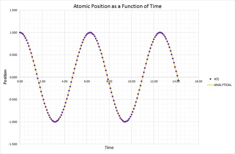
As you can see, the two methods are in very close agreement. The harmonic oscillator values were calculated using the following equation: $x(t)=Acos(\omega t+\varphi )$

where $A=1,\omega =1$ and $\varphi =0$.

The total energy of the oscillator for the velocity-Verlet solution is equal to the sum of the kinetic and potential energies, as outlined in the following graph:

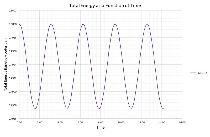
The potential energy term was found using the equation $E_{pot}=\frac{1}{2}k{x}^2$, where the force constant,$k$, is equal to 1. The kinetic energy term was calculated using $E_{kin}=\frac{1}{2}m{v}^2$, where the mass, $m$ is equal to 1.

Below is a plot showing the difference (error) between the results from the harmonic oscillator and the velocity-Verlet algorithm:

As time increases, the maximum in the error also increases. This is due to the harmonic oscillator having a slightly shorter wavelength than the one contained in the algorithm, so as each period of the wave passes, this difference increases. This relationship is highlighted in the following graph where the peak maxima of the error are plotted against time:

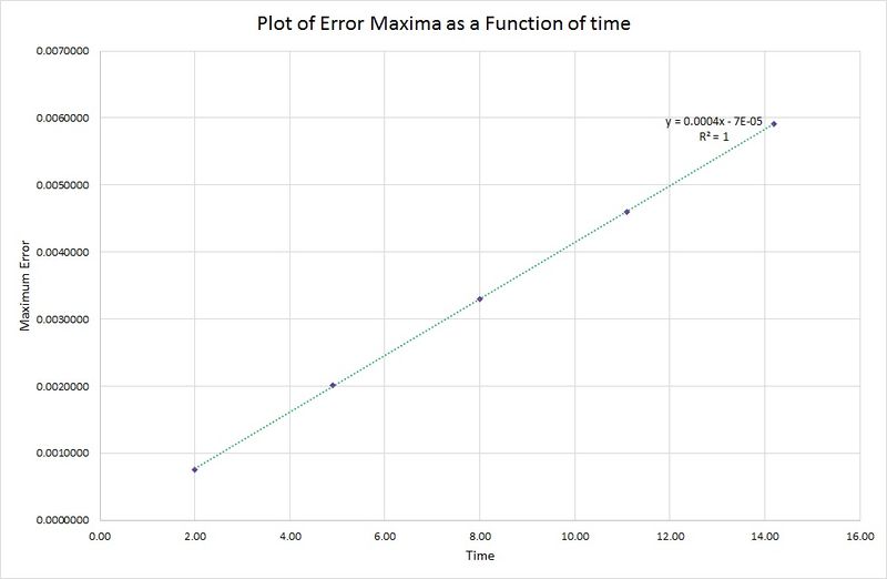
There is a linear relationship between the error data for the harmonic oscillator and the algorithm, therefore the period of oscillation in the position/time graph must be constant.

Atomic Forces

The force acting on an object is governed by the potential that it experiences: ${\mathbf{F}}_i=-\frac{\mathrm{d}U({\mathbf{r}}^N)}{\mathrm{d}{\mathbf{r}}_i}$

Single Lennard-Jones interaction: $\varphi (r)=4ϵ(\frac{{\sigma }^{12}}{r^{12}}-\frac{{\sigma }^6}{r^6})$

The separation at which the potential energy is zero can be found by equating the single Lennard-Jones interaction to zero, and solving for $r$. The following results:

  $r_0=\sigma$

The force at this separation is found by differentiating the L-J potential, and leads to this result:

  $\mathbf{F}(r_0)=\frac{24ϵ}{\sigma }$

To find the equilibrium separation, the derivative of the potential energy is set to zero and solved for $r$:

  $r_{eq}=\sqrt[6]{2}\sigma$

The well depth is equal to the potential energy at the equilibrium separation and thus can be found by substituting the value for $r_{eq}$ into the L-J potential equation and rearranging:

  $\varphi (r_{eq})=-ϵ$

Evaluation of the following integrals when $\sigma =ϵ=1.0$ leads to:

  $\underset{2\sigma }{\overset{\mathrm{\infty }}{\int }}\varphi (r)\mathrm{d}r=-0.025$

  $\underset{2.5\sigma }{\overset{\mathrm{\infty }}{\int }}\varphi (r)\mathrm{d}r=-0.0082$

  $\underset{3\sigma }{\overset{\mathrm{\infty }}{\int }}\varphi (r)\mathrm{d}r=-0.0033$

Periodic Boundary Conditions

Taking the concentration of water under standard conditions to be $$\begin{gathered} 55 \\ mol \\ d{m}^{-3} \end{gathered}$$, the number of water molecules in 1 ml of water under standard conditions is therefore approximately $3.3\times 10^{22}$. The volume of 10000 water molecules under standard conditions is approximately $$\begin{gathered} 3.0\times 10^{-19} \\ ml \end{gathered}$$. As you can see, this is a remarkably small volume: too small to be measured in a laboratory environment. This illustrates in a real world application just how small a typical simulation is (where the number of particles, $N$, is normally between $1000$ and $10000$).

An atom at position $(0.5,0.5,0.5)$ in a cubic simulation box, which runs from $(0,0,0)$ to $(1,1,1)$ along the vector $(0.7,0.6,0.2)$ in a single timestep, will end up at the point $(0.2,0.1,0.7)$ once the periodic boundary conditions have been applied.

Periodic boundary conditions result in a simulation of an infinite lattice, which when calculating the potential would include an infinite number of pair interactions. This is both impractical for the simulations and unnecessary because after a certain interatomic distance, the integral of the Lennard-Jones potential becomes negligible, thus a cutoff value is applied. The three example integrals given above show the insignificance of the energy contribution when integrating from the cutoff value to infinity.

Reduced Units

By convention, reduced units are used when working with Lennard-Jones interactions; all quantities are divided by scaling factors. This converts values into convenient forms from what would otherwise be rather lengthy (e.g. distances are divided by $\sigma$, generating a value that's typically around $1$ instead of $1\times 10^{-10}$).

These reduced units are denoted by an asterisk, and undergo the following conversions:

  Distance: $r^{*}=\frac{r}{\sigma }$
  Energy: $E^{*}=\frac{E}{ϵ}$
  Temperature: $T^{*}=\frac{k_{B}T}{ϵ}$

For Argon, the Lennard-Jones parameters are $$\begin{gathered} \sigma =0.34 \\ nm \end{gathered}$$ and $$\begin{gathered} \frac{ϵ}{k_B}=120 \\ K \end{gathered}$$.

The LJ cutoff is $r^{*}=3.2$, which in real units is $$\begin{gathered} (3.2\times 0.34)=1.1 \\ nm \end{gathered}$$.

The well depth is $$\begin{gathered} \varphi (r_{eq})=-ϵ=-120\times k_B=-1.7\times 10^{-21}J=-1.0 \\ kJ \\ mo{l}^{-1} \end{gathered}$$.

The reduced temperature $T^{*}=1.5$. In real units, $$\begin{gathered} T=(1.5\times 120)=180 \\ K \end{gathered}$$.

Equilibration

The Simulation Box

Before an MD simulation can take place, the initial states of all the atoms in that system must be known. These defined states can vary depending on the method of numerical integration required, but as a general rule, at least the starting position of each atom needs to be specified. LAMMPS is able to generate crystal lattice structures according to the associated input command; for a solid crystal this is reasonably simple, whereas it becomes more complicated to generate coordinates for atoms contained in a liquid. The Brownian motion of a liquid results in an absence of long-range order, meaning that there is no single point of reference from which to work out the positions of all other atoms. Giving atoms random starting coordinates would cause problems in simulations because there is a possibility of several atoms being assigned coordinates in such close proximity that they overlap. Atomic overlap of this nature would generate huge repulsion potentials and raise the energy of the system by an amount unrepresentative of a real liquid system.

Formation of a simple cubic lattice, although an unlikely situation for the system to be found physically, provides a starting point for the simulations. The command:

lattice sc 0.8

creates a grid of points which form the simple cubic lattice, consisting of one lattice point per unit cell. The value of $0.8$ specifies the number density, which is the number of lattice points per unit volume. Thus:

  $$\begin{gathered} volume \\ of \\ unit \\ cell=\frac{lattice \\ points \\ per \\ unit \\ cell}{number \\ density} \end{gathered}$$

From the output file of a simulation, the following line could be seen:

Lattice spacing in x,y,z = 1.07722 1.07722 1.07722

This corresponds to the distance (in reduced units) between points of the specified lattice type. Using a rearrangement of the above formula, it can be seen how this lattice spacing corresponds to a number density of $0.8$:

$$\begin{gathered} \frac{lattice \\ points \\ per \\ unit \\ cell}{(lattice \\ spacing{)}^3}=number \\ density; \\ \frac{1}{1.07722^3}=0.8 \end{gathered}$$

If instead we consider a face-centred cubic (fcc) lattice (which has 4 lattice points) with a number density of $1.2$, the side length of the cubic unit cell becomes:

$\sqrt[3]{\frac{4}{1.2}}=1.4938$

An input command of:

region box block 0 10 0 10 0 10
create_box 1 box
create_atoms 1 box

would generate a simulation box consisting of 1000 (10x10x10) unit cells of the lattice type being used. Considering an fcc lattice again, this would correspond to 4000 atoms being generated, as there are 4 atoms per unit cell.

Defining Atomic Properties

Along with the positions of the atoms, their physical properties are also needed for a successful simulation.

The following commands appear in the input script:

mass 1 1.0
pair_style lj/cut 3.0
pair_coeff * * 1.0 1.0

The first of these corresponds to the mass of atoms of type 1, the value of which is 1.0. The second line specifies the type of interactions between pairs of atoms; in this case the interaction type is the Lennard-Jones potential. The "cut 3.0" refers to the cutoff point of the Lennard-Jones potential; any interactions beyond $3\sigma$ are not considered. In the final line, "pair_coeff" relates to $ϵ$ and $\sigma$, respectively, with " * * " meaning that the entire system of atoms are to be considered. "1.0 1.0" are the values of the specified parameters.

One more property still needs to be defined: the velocity of each atom. Given that ${\mathbf{x}}_i(0)$ and ${\mathbf{v}}_i(0)$ are being specified, the velocity Verlet integration algorithm needs to be implemented.

Running the Simulation

The following lines instruct LAMMPS to input a timestep value of 0.001 whenever it encounters the text "${timestep}" on a subsequent line.

### SPECIFY TIMESTEP ###
variable timestep equal 0.001
variable n_steps equal floor(100/${timestep})
variable n_steps equal floor(100/0.001)
timestep ${timestep}
timestep 0.001

### RUN SIMULATION ###
run ${n_steps}
run 100000

Although this may seem rather a long instruction, it is considerably easier to use this variable definition of the timestep, rather than just using:

timestep 0.001
run 100000

If only these two lines of code were used, changing the timestep would require manual modification at every point it appears in the script. The variable version only requires the first input value to be changed, whilst also ensuring that the overall length of time for the simulation is kept constant, no matter what the value of the timestep is.

Checking Equilibrium

By plotting the thermodynamic data from a simulation output, it can be seen whether or not a system reaches the equilibrium state, and if so, how long it takes to get there. The following graphs show these equations of state, alongside a magnified snapshot to ease analysis:

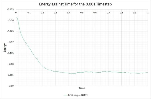
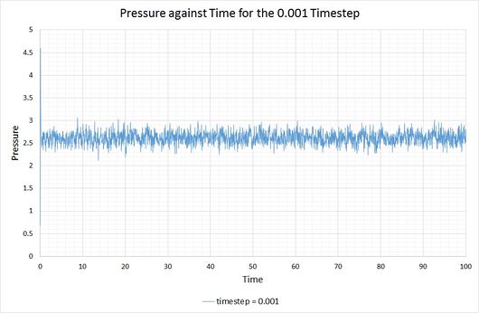
From these graphs it is shown that the simulation does indeed reach equilibrium with a timestep of 0.001, as a constant (average) value is maintained for the energy, temperature and pressure of the system. From investigation of the magnified graphs, the time at which the equilibrium state is reached can be identified. It appears to vary slightly between the three parameters, therefore we will select the value corresponding to the latest point in time, this being for the energy plot at approximately $t=0.3$.

Now let's compare the energies of a system simulated with different timesteps:

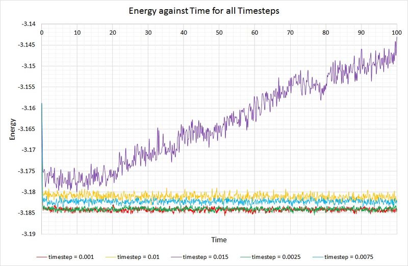
Shorter timesteps produce results which more accurately describe the physical reality of a simulation. However, this comes at a cost; the same number of simulation steps cover a shorter amount of real time compared to larger timesteps, limiting the length of observation. The largest timestep which generates reasonable results is 0.01, because the system has been able to reach equilibrium. In contrast, the 0.015 timestep (the largest of them all) has failed to reach the equilibrium state and is therefore a particularly bad choice of timestep for simulation. The best choice of timestep here would be 0.0025 because its energy is most comparable to that produced by 0.001 (the smallest timestep producing the most accurate results), whilst providing a longer overall simulation time.

Running Simulations Under Specific Conditions

Ensembles

Up until this point, the simulations have been described by a microcanonical ensemble (also know as NVE ensemble), derived from statistical mechanics. The macroscopic variables N (total number of atoms), V (volume of the system) and E (total energy) are held constant.

The following simulations have been modified to run under the conditions of an isobaric-isothermal (NpT) ensemble, leading to an equation of state for the model fluid at atmospheric pressure.

Thermostats and Barostats

According to the equipartition theorem from statistical thermodynamics, every degree of freedom in a system at equilibrium will, on average, have $\frac{1}{2}{k}_{B}T$ of energy. In a system consisting of $N$ atoms, each with 3 degrees of freedom, the following equations for kinetic energy are obtained:

$E_K=\frac{3}{2}N{k}_{B}T$

$\frac{1}{2}\sum _i{m}_i{v}_i^2=\frac{3}{2}N{k}_{B}T$

From this, the instantaneous temperature, $T$, can be determined after every timestep. $T$ will fluctuate and differ from the target temperature, $\mathfrak{𝔗}$, specified in the input script. Changing the temperature by multiplying by a constant factor $(\gamma )$ enables the kinetic energy of the system to be controlled:

• If $T>\mathfrak{𝔗}$, then $E_K$ is too high and needs to be reduced $(\gamma <1)$
• If $T<\mathfrak{𝔗}$, then $E_K$ is too low and needs to be increased $(\gamma >1)$

In order to ensure that the temperature is correct $(T=\mathfrak{𝔗})$, a solution for $\gamma$ must be determined. This can be done by solving the following equations:

$\frac{1}{2}\sum _i{m}_i{v}_i^2=\frac{3}{2}N{k}_{B}T$

$\frac{1}{2}\sum _i{m}_i(\gamma v_i{)}^2=\frac{3}{2}N{k}_B\mathfrak{𝔗}$

The solution:

→ $\frac{1}{2}\sum _i{m}_i(\gamma v_i{)}^2=\frac{1}{2}{\gamma }^2\sum _i{m}_i{v}_i^2={\gamma }^2\frac{3}{2}N{k}_{B}T$

→ ${\gamma }^2\frac{3}{2}N{k}_{B}T=\frac{3}{2}N{k}_B\mathfrak{𝔗}$

→ ${\gamma }^{2}T=\mathfrak{𝔗}$

Thus:

  $\gamma =\sqrt{\frac{\mathfrak{𝔗}}{T}}$

To control the pressure of the system, the pressure is calculated at each timestep and if it is too high, the size of the simulation box is increased. Similarly, the box is decreased if the pressure is too low. For this reason, the volume of the simulation box is not constant, thus the simulations are in the NpT ensemble.

Examining the Input Script

The following lines are taken from one of the input scripts:

fix aves all ave/time 100 1000 100000 v_dens v_temp v_press v_dens2 v_temp2 v_press2
run 100000

The fix command tells LAMMPS which simulated thermodynamic properties to compute and generates the average value for each one. The three numbers that follow (100 1000 100000) relate to the frequency of sampling (Nevery, i.e. use input values every 100 timesteps), the number of samples to incorporate in the average (Nrepeat, i.e. use input values 1000 times for calculating averages) and how frequently to calculate the averages (Nfreq, i.e. calculate averages every 100000 timesteps).

The second line (run 100000) dictates how long to run the simulation for; as the timestep has been set at 0.0025, the simulation will run for 250 units of reduced time.

Plotting the Equations of State

From rearrangement of the ideal gas law, the density $\left(\frac{N}{V}\right)$ can be determined:

$pV=N{k}_{B}T$ → $\frac{N}{V}=\frac{p}{k_{B}T}$

As all calculations are performed using reduced units, $k_B=1$ in this instance, therefore the expression for density simplifies to:

  $\frac{N}{V}=\frac{p}{T}$

The following graph displays the densities plotted as a function of temperature for the two pressures simulated (2.5 and 3.0), as well as the densities predicted by the ideal gas law at the same pressures. Whilst the experimental data points include error bars for both parameters plotted, the ones for the densities are not visible as the standard error is so small (approx. +/-0.004 reduced density units). Looking at the temperature error bars, it can be seen that the standard error increases with increasing temperature.

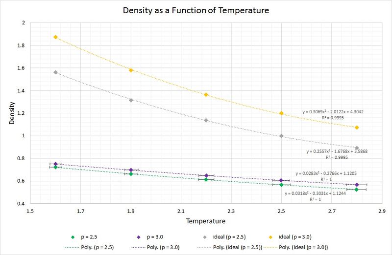
The data from the simulations produce densities which are considerably lower than those predicted by the ideal gas law. This can be rationalised by the fact that the ideal gas law makes a series of assumptions, including an absence of intermolecular interactions. In the simulations of the liquid these assumptions have not been made, and instead, Lennard-Jones interactions such as short-range repulsions arising from orbital overlap between atoms, are taken into account. As a result of this, the atoms are found to be at a greater separation, thus the density is lower.

As the pressure is increased from 2.5 to 3.0, the discrepancy between the ideal and simulated data increases. This can be attributed to the aforementioned short-range repulsions which are more prevalent in a higher pressure system, as the atoms are closer together on average, and thus experience a greater repulsion. Moreover, at the higher pressure of 3.0, the assumptions made by the ideal gas model result in a greater deviation from the simulated data than that found with the pressure of 2.5.

One other observation is the convergence between the simulated and ideally predicted data as the temperature increases. A rise in temperature leads to a rise in kinetic energy; $E_K$ begins to dominate and as it does so, the intermolecular repulsions become increasingly negligible. Consequently, the ideal gas law begins to describe the system more accurately.

Heat Capacity

Below is an example of one the input scripts used to simulate a liquid in density-temperature $({\rho }^{*},T^{*})$ phase space, in order to calculate the heat capacity. The simulations were run under the NVT ensemble.

### DEFINE SIMULATION BOX GEOMETRY ###
lattice sc 0.2
region box block 0 15 0 15 0 15
create_box 1 box
create_atoms 1 box

### DEFINE PHYSICAL PROPERTIES OF ATOMS ###
mass 1 1.0
pair_style lj/cut/opt 3.0
pair_coeff 1 1 1.0 1.0
neighbor 2.0 bin

### SPECIFY THE REQUIRED THERMODYNAMIC STATE ###
variable T equal 2.0
variable timestep equal 0.0025

### ASSIGN ATOMIC VELOCITIES ###
velocity all create ${T} 12345 dist gaussian rot yes mom yes

### SPECIFY ENSEMBLE ###
timestep ${timestep}
fix nve all nve

### THERMODYNAMIC OUTPUT CONTROL ###
thermo_style custom time etotal temp press
thermo 10

### RECORD TRAJECTORY ###
dump traj all custom 1000 output-1 id x y z

### SPECIFY TIMESTEP ###

### RUN SIMULATION TO MELT CRYSTAL ###
run 10000
unfix nve
reset_timestep 0

### BRING SYSTEM TO REQUIRED STATE ###
variable tdamp equal ${timestep}*100
fix nvt all nvt temp ${T} ${T} ${tdamp}
run 10000
unfix nvt
fix nve all nve
reset_timestep 0

### MEASURE SYSTEM STATE ###
thermo_style custom step etotal temp press density
variable temp equal temp
variable etotal equal etotal
variable etotal2 equal etotal*etotal
fix aves all ave/time 100 1000 100000 v_temp v_etotal v_etotal2
run 100000

variable avetemp equal f_aves[1]
variable aveetotal equal f_aves[2]
variable aveetotal2 equal f_aves[3]
variable cv equal (v_aveetotal2-v_aveetotal*v_aveetotal)/(v_avetemp*v_avetemp)*atoms*atoms/vol

print "Averages"
print "--------"
print "Temperature: ${avetemp}"
print "Heat Capacity: ${cv}"

According to statistical thermodynamics, the heat capacity of a system can be determined from the magnitude of the fluctuations about the average equilibrium value for the total energy, whilst the temperature is held 'constant'. The following equation describes this relationship:

$C_V=\frac{\partial E}{\partial T}=\frac{\mathrm{V}\mathrm{a}\mathrm{r}[E]}{k_B{T}^2}=N^2\frac{⟨E^2⟩-⟨E{⟩}^2}{k_B{T}^2}$

$N$ is the number of atoms and $\mathrm{V}\mathrm{a}\mathrm{r}[E]$ is the variance in $E$ which relates to the fluctuation about equilibrium.

The graph below shows that an increase in density leads to an increase in the isochoric heat capacity:

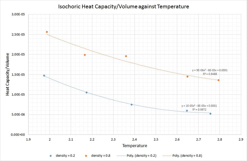
This is as you would expect, because a system of fixed volume with a higher density contains more atoms, thus a greater amount of thermal energy is required to raise the temperature of the system by the same amount as that of a lower density.

Perhaps surprisingly, the heat capacity decreases as the temperature increases. One rationale for this is that at higher temperatures there is an increase in the density of states for the system (i.e. there are a greater number of occupationally available states per interval of energy at each energy level). This means that heat transfer to the system is made more facile as less energy is needed to proportionally populate each energy level.

Radial Distribution Function

In order to ascertain what values of temperature and density to use for the simulations of solid, liquid and vapour phases of the Lennard-Jones system, a phase diagram for the Lennard-Jones system was analysed. To make the results more comparable, the selected temperature was kept at 1.2 (in reduced units) for all three phases. The corresponding densities were as follows:

Vapour density = 0.01

Liquid density = 0.8

Solid density = 1.2

The output trajectory files from these simulations were used to calculate the radial distribution functions (RDFs).

The RDF describes the probability that an atom can be found at a certain distance from a reference atom; it is an indication of any long-range order within a system.

The following graph shows the RDFs for the vapour, liquid and solid phases from the simulations:

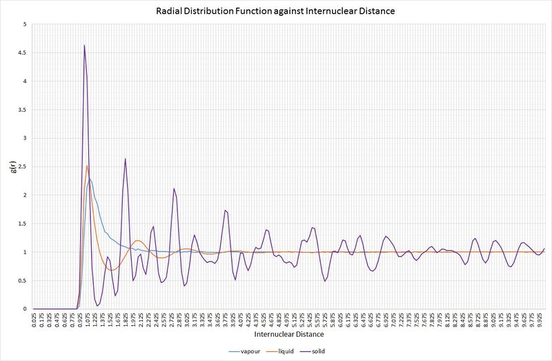
Comparison of the RDFs for each of the three systems highlights some key structural features. Firstly, the vapour phase holds no long-range order, as indicated by the fact that it only has one maximum in the RDF, rapidly decaying to a minimum (at $g(r)=1$) beyond an internuclear separation greater than approximately 1.2. For the liquid phase, there are three distinct maxima whose amplitudes significantly decrease with increasing internuclear separation. This decrease in amplitude as the RDF approaches one is representative of an absence of long-range order within the system, but it is more ordered than the vapour. In a solid, the RDF has an infinite number of sharp peaks, the separations and heights of which are characteristic of its lattice structure. The solid simulated here demonstrates the RDF of an fcc lattice. Over the range of the simulation, a constant minimum has not been reached, signifying considerable long-range order, as one would expect for a solid. At short distances (less than one atomic diameter) $g(r)=0$ for all three phases; the probability of finding two atoms at or below this separation is zero. This is a result of the strong repulsive forces between atoms. The varying peak broadness between phases is also significant; the solid RDF exhibits the narrowest peaks because a solid experiences minimal random atomic motion compared to a liquid and a vapour.

An experimental determination of the RDF can be carried out using X-ray diffraction, via analysis of the diffraction patterns. A solid would generate an X-ray diffraction pattern with bright, sharp spots, characteristic for the regular arrangement of atoms in a crystal, whilst a liquid would create a pattern with regions of low and high intensity without sharp spots. Such experimental distribution functions could then be compared to those generated by simulations.

Lattice sites, lattice spacing and coordination numbers can be determined from the RDF peaks. We will take the first three peaks of the solid RDF to illustrate this:

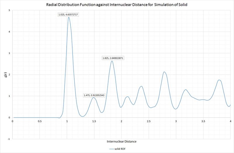
Intuitively, one would expect these peaks to correspond to the three shortest interatomic distances within the unit cell of an fcc lattice. Below is a scheme illustrating this unit cell, and the corresponding distances:

A, B and C are at distances of 1.025, 1.475 and 1.825, respectively, from the reference atom. The lattice spacing is therefore 1.475 as B corresponds to the length of the unit cell. The coordination numbers can be found by inspection of the unit cell, or by inspection of the integral of the RDF, as shown in the following graph:

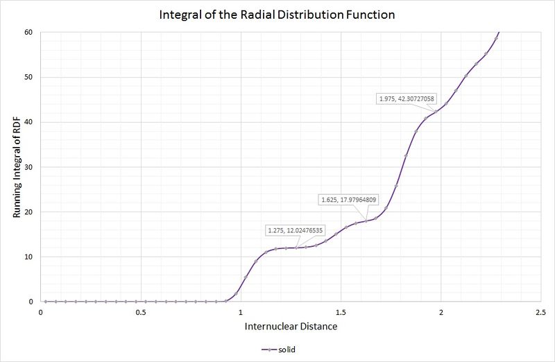
The first coordination sphere (A) consists of 12 atoms, which can be read from the first highlighted point on the graph where the curve plateaus. The second coordination sphere (B) contains 6 atoms; the integral is a running total, therefore the number of atoms from the previous sphere need to be subtracted (i.e. 18 - 12 = 6). The final sphere (C) contains 24 atoms, by the same method.

Dynamical Properties and the Diffusion Coefficient

The diffusion coefficient, $D$, describes the movement ability of atoms in a system. In the discussion that follows, two different methods have been used to determine $D$: mean squared displacement and velocity autocorrelation function.

The temperature and density parameters used were the same as in the previous section:

Temperature = 1.2 for all three phases

Vapour density = 0.01

Liquid density = 0.8

Solid density = 1.2

Mean Squared Displacement

$D$ is related to the mean squared displacement (MSD) by the following equation:

$D=\frac{1}{6}\frac{\partial ⟨r^2(t)⟩}{\partial t}$

To get the final value for $D$ we must divide by the simulation timestep, which in this case is 0.002.

As you can see, there is not a particularly good agreement between the linear fit and the vapour phase plot for MSD against timestep:

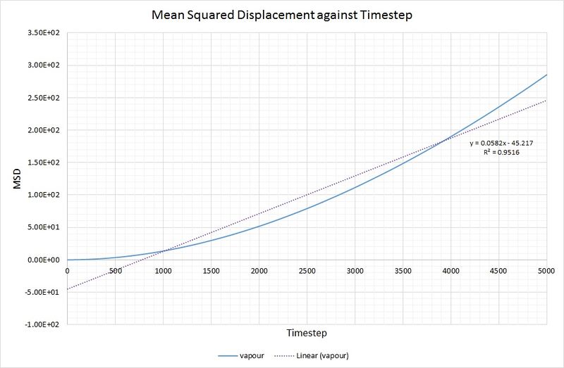
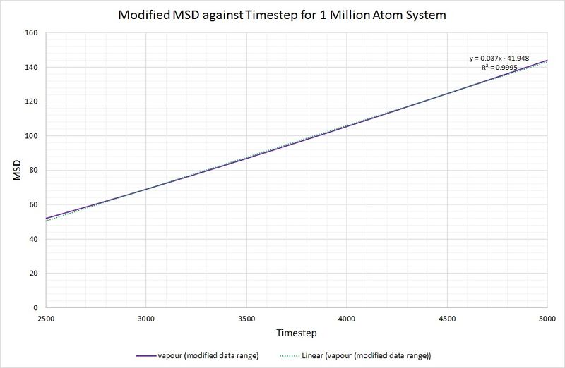
To rectify this, making the calculation of $D$ more accurate, the data range used has been limited to 2500-5000 for the timestep:

Now that the linear fit is more appropriate (as indicated by a higher value of R squared), we can calculate $D_v$ by taking the gradient of the line, dividing by the timestep and multiplying by $\frac{1}{6}$:

$D_v=\frac{1}{6}\frac{0.0827}{0.002}=6.89$

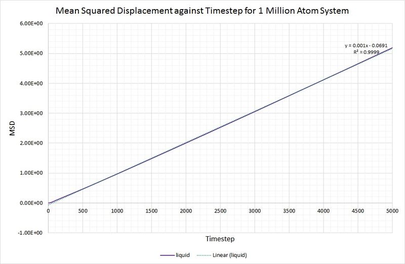
The same method is used to determine the diffusion coefficient for the liquid ($D_l$), but without the need for data range modification:

$D_l=\frac{1}{6}\frac{0.001}{0.002}=0.0833$

This value is considerably lower than that obtained for the vapour phase, which is as you would expect because a gas is far less dense than a liquid, and the gaseous atoms can therefore diffuse much further and more easily.

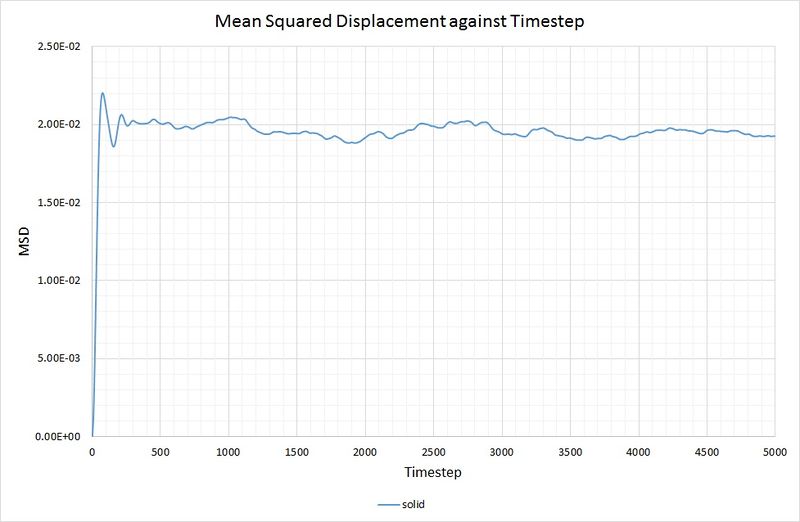
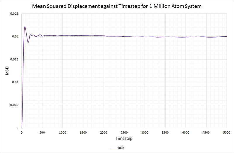
For the solid phase, the gradient of the curve fluctuates, but is approximately zero, thus $D_s\approx 0$. Again, this is as you would expect, because the atoms in a solid have some motion as they vibrate, but they cannot diffuse through the crystal because each one collides with its nearest neighbours. The graph for the solid phase MSD is shown below:

For comparison, the same method has been employed on the data generated by a larger system containing 1,000,000 atoms. The graphs can be seen below:

Summary of diffusion coefficients for both systems:

	8,000 atom system, $$\begin{gathered} D/ \\ {s}^{-1} \end{gathered}$$	1,000,000 atom system, $$\begin{gathered} D/ \\ {s}^{-1} \end{gathered}$$
Lennard-Jones vapour	6.89	3.08
Lennard-Jones liquid	0.0833	0.0833
Lennard-Jones solid	0	0

$D_s\approx 0$ for both the small and large system. As mentioned before, this is because the function of the MSD reaches an average constant value (around 0.02). A zero gradient means that an infinite amount of time is needed for the atoms to vary their MSD, thus it can be deduced that there is approximately no diffusion in the solid in either simulation.

The two systems result in the same value for $$\begin{gathered} D_l \\ (0.0833) \end{gathered}$$. From this, it can be deduced that 8,000 atoms is a large enough system to generate accurate results.

There is a large disagreement between the values of $D_v$, most likely arising from a difference in density between the two simulations. A higher diffusion coefficient relates to a lower density as particles can diffuse more rapidly, thus the smaller system here has a lower density. Both graphs for the vapour phase MSDs have an initial non-linear trend. This is a result of the particles' momenta initially dominating over the time-dependent diffusion coefficient. As more time passes, the systems equilibrate as $D$ becomes constant, and the graphs begin to display linearity.

Velocity Autocorrelation Function

Our second method for determining $D$ involves using the velocity autocorrelation function (VACF). The VACF describes the change in velocity of an atom with respect to time. The time at which the velocity becomes uncorrelated is denoted as $\tau$, and is the difference between the velocity at time $t+\tau$ and time $t$. The integral of this function is what leads to determining the diffusion coefficient.

Normalised VACF for a 1D Harmonic Oscillator

The VACF:

$C(\tau )=⟨\mathbf{v}(t)\cdot \mathbf{v}(t+\tau )⟩$

This can also be written as:

$C(\tau )=\frac{\underset{-\mathrm{\infty }}{\overset{\mathrm{\infty }}{\int }}v(t)v(t+\tau )\mathrm{d}t}{\underset{-\mathrm{\infty }}{\overset{\mathrm{\infty }}{\int }}{v}^2(t)\mathrm{d}t}$

The equation defining position in a classical harmonic oscillator can be used to solve the VACF, first by differentiating to get the equation for velocity:

  $x(t)=Acos(\omega t+\varphi )$

  $v(t)=\frac{\mathrm{d}x(t)}{\mathrm{d}t}=-\omega Asin(\omega t+\varphi )$

We also need the following expressions to substitute into the integral:

  $v(t+\tau )=-\omega Asin[\omega (t+\tau )+\varphi ]$

  $v^2(t)={\omega }^2{A}^{2}si{n}^2(\omega t+\varphi )$

Substituting these identities into the equation for the VACF gives:

$C(\tau )=\frac{\underset{-\mathrm{\infty }}{\overset{\mathrm{\infty }}{\int }}\omega Asin(\omega t+\varphi )\omega Asin[\omega (t+\tau )+\varphi ]\mathrm{d}t}{\underset{-\mathrm{\infty }}{\overset{\mathrm{\infty }}{\int }}{\omega }^2{A}^{2}si{n}^2(\omega t+\varphi )\mathrm{d}t}$

which can be simplified to:

$C(\tau )=\frac{\underset{-\mathrm{\infty }}{\overset{\mathrm{\infty }}{\int }}sin(a)sin(a+b)\mathrm{d}a}{\underset{-\mathrm{\infty }}{\overset{\mathrm{\infty }}{\int }}si{n}^2(a)\mathrm{d}a}$

where:

  $a=\omega t+\varphi$
  $b=\omega \tau$

Using the trigonometric identity:

  $sin(a+b)=sin(a)cos(b)+cos(a)sin(b)$

the following expression is obtained:

$C(\tau )=\frac{\underset{-\mathrm{\infty }}{\overset{\mathrm{\infty }}{\int }}sin(a)[sin(a)cos(b)+cos(a)sin(b)]\mathrm{d}a}{\underset{-\mathrm{\infty }}{\overset{\mathrm{\infty }}{\int }}si{n}^2(a)\mathrm{d}a}$

which simplifies to:

$C(\tau )=cos(b)+sin(b)\frac{\underset{-\mathrm{\infty }}{\overset{\mathrm{\infty }}{\int }}sin(a)cos(a)\mathrm{d}a}{\underset{-\mathrm{\infty }}{\overset{\mathrm{\infty }}{\int }}si{n}^2(a)\mathrm{d}a}$

The trigonometric identities:

  $sin(2a)=2sin(a)cos(a)$
  $cos(2a)=1-2si{n}^2(a)$

are then rearranged for $sin(a)cos(a)$ and $si{n}^2(a)$, respectively, and substituted into the previous equation:

$C(\tau )=cos(b)+sin(b)\frac{\underset{-\mathrm{\infty }}{\overset{\mathrm{\infty }}{\int }}\frac{1}{2}sin(2a)\mathrm{d}a}{\underset{-\mathrm{\infty }}{\overset{\mathrm{\infty }}{\int }}\frac{1}{2}[1-cos(2a)]\mathrm{d}a}$

Sine is an odd function, therefore its integral over infinite space is zero and this term cancels out of the equation, leading to the final result for the normalised velocity autocorrelation function for a 1D harmonic oscillator:

  $C(\tau )=cos(b)=cos(\omega \tau )$

Diffusion Coefficients from VACF

The simulations performed previously for the MSD also provided data for the VACF, thus calculations of $D$ for the solid, liquid and vapour phases have been done for both the 8,000 atom system and the 1,000,000 atom system.

The VACFs for the solid and liquid from the 8,000 atom system were plotted against timestep, also with the VACF for the classical harmonic oscillator, with $\omega =1/2\pi$:

It can be seen from this graph that the correlation between velocities for the liquid and solid decreases as time passes, which is a result of collisions between particles. The Lennard-Jones solid experiences a few oscillations about VACF = 0, with a decrease in amplitude each time. This damped oscillation arises due to the frequent collisions. The Lennard-Jones liquid displays only one minimum as particle collisions are less frequent for a system of lower density.

Van der Waals forces of attraction occur between atoms of intermediate distance in the Lennard-Jones solid and liquid, which result in repulsions when the atoms get too close, but it is the collisions between atoms that cause a change in velocity, leading to the minima in the graphs when the product of the velocities is at a maximum (but negative due to the opposing directions).

There are no collisions involved for a harmonic oscillator, hence it oscillates periodically without being damped and looks vastly different to the liquid and solid VACFs.

The VACF for the vapour phase is absent here, because it would simply give an almost perfectly horizontal line. This is because the vapour is so diffuse that no collisions would occur in the time-frame under study.

The diffusion coefficient is related to the VACF by the following equation:

$D=\frac{1}{3}\underset{0}{\overset{\mathrm{\infty }}{\int }}C(\tau )\mathrm{d}\tau$

By plotting a running integral of the VACF (using the trapezium rule) against timestep, the final value can be used to determine the diffusion coefficient. The following graphs were obtained for the system of 8,000 atoms and the 1,000,000 atom system:

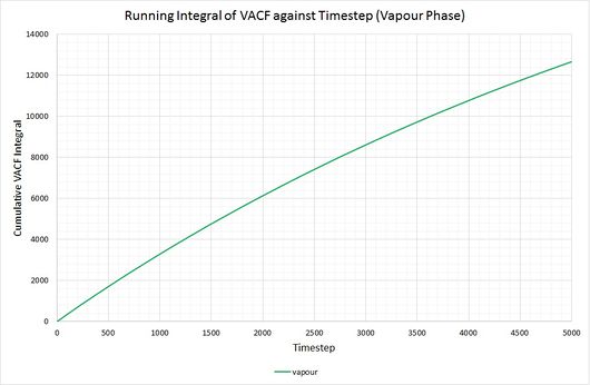
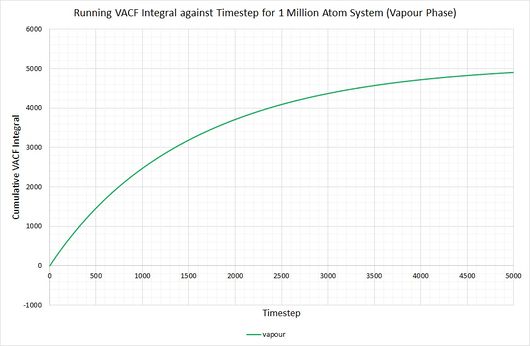
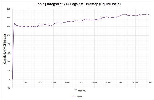
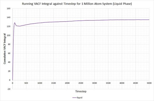
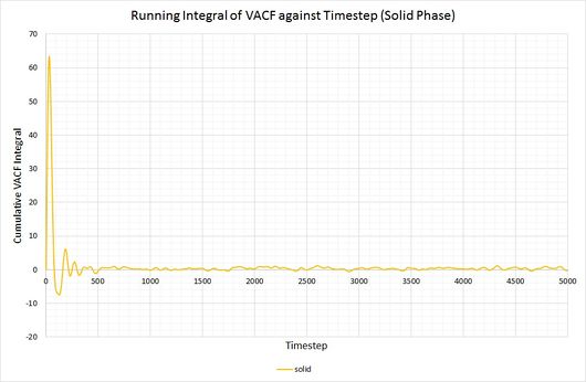
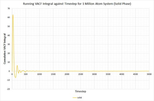
By taking the final value of each running integral, dividing by 3 and multiplying by 0.002 (to correct for the timestep), the following diffusion coefficients were obtained:

	8,000 atom system, $$\begin{gathered} D/ \\ {s}^{-1} \end{gathered}$$	1,000,000 atom system $$\begin{gathered} D/ \\ {s}^{-1} \end{gathered}$$
Lennard-Jones vapour	8.45	3.27
Lennard-Jones liquid	0.0979	0.0901
Lennard-Jones solid	approx. 0	approx. 0

The largest source of error when determining $D$ for the two systems is that it is assumed they take the same amount of time to converge. This is particularly prominent in the case of the vapour phase where you can clearly see that the simulation run with 1,000,000 atoms has converged much more considerably than the one run with 8,000. The values for $D_v$ also show the least agreement, which reflects this error.

As before, the diffusion coefficient for both solids equates to approximately zero, employing the same rationale as with the MSD.

The two methods for determining $D$ are in reasonably good agreement with each other.