Rep:Mod:ym28142814

Theory

Velocity Verlet Algorithm

The velocity-Verlet solution for the position at time t is calculated by the equation below where timestep is 0.1:

${\mathbf{x}}_i(t+\delta t)={\mathbf{x}}_i\left(t\right)+{\mathbf{v}}_i(t+\frac{1}{2}\delta t)\delta t$

The position of a classical harmonic oscillator is calculatd by $x(t)=A\cos (\omega t+\varphi )$. In this case, $A$=1.00, $\varphi$=0.00 and $\omega$=1.00.

Figure 1:classical solution and velocity-Verlet solution for the position at time t

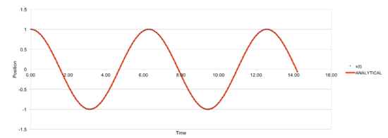
The plot above shows a comparison between the classical solution and velocity-Verlet solution and it can be seen that there are no significant differences between two solutions.

The graph below shows the actual difference between the two solutions.

Figure 2:absolute difference between "ANALYTICAL" and velocity-Verlet solution

The maxima in error are estimated and shown as a function of time (brown line), which can be fit to the equation shown in the graph. The total energy of the oscillator is the sum of kinetic and potential energies: $E=\frac{m{v}^2}{2}+\frac{k{x}^2}{2}$, where $v$and $x$ are the velocity-Verlet solution for velocity and position ($m$=1.00 and $k$=1.00).

Figure 3:total energy and its lower and upper limit when timestep is 0.1

Figure 4:total energy and its lower and upper limit when timestep is 0.2

In order to make sure the total energy does not change by more than 1%, timestep should be no more than 0.2. In a simple harmonic oscillator, the sum of kinetic energy and potential energy should ideally be constant, so it is important to monitor the total energy of a physical system when modeling its behaviour numerically.

Atomic Forces

For a single Lennard-Jones interaction, the potential energy can be calculated by $\varphi \left(r\right)=4ϵ(\frac{{\sigma }^{12}}{r^{12}}-\frac{{\sigma }^6}{r^6})$. When the potential energy is zero, the separation $r_0$ is equal to the value of $\sigma$ ($r_0$ = $r$=$\sigma$).

The force acting on an object is determined by the potential that it experiences:

${\mathbf{F}}_i=-\frac{\mathrm{d}U\left({\mathbf{r}}^N\right)}{\mathrm{d}{\mathbf{r}}_i}$

So the force at this seperation $r_0$ can be calculated as below:

${\mathbf{F}}_i=-\frac{\mathrm{d}\varphi \left(r_i\right)}{\mathrm{d}{\mathbf{r}}_i}$

$\mathbf{F}=-\frac{\mathrm{d}4ϵ(\frac{{\sigma }^{12}}{r^{12}}-\frac{{\sigma }^6}{r^6})}{\mathrm{d}\mathbf{r}}$

$\mathbf{F}=-4ϵ(\frac{-12{\sigma }^{12}}{r^{13}}+\frac{6{\sigma }^6}{r^7})$

Since $r_0$ = $r$=$\sigma$,

$\mathbf{F}=-4ϵ(\frac{-12r_0^{12}}{r_0^{13}}+\frac{6r_0^6}{r_0^7})$

Therefore the force at $r_0$ can be simplified to :

$\mathbf{F}=\frac{24ϵ}{r_0}$

The equilibrium separation can be found when the force is equal to zero:

$\mathbf{F}=-4ϵ(\frac{-12{\sigma }^{12}}{r^{13}}+\frac{6{\sigma }^6}{r^7})=0$

$r_{eq}=\sqrt[6]{2}\sigma$

Since $\varphi \left(r_{eq}\right)=4ϵ(\frac{{\sigma }^{12}}{r_{eq}^{12}}-\frac{{\sigma }^6}{r_{eq}^6})$, the well depth $ϵ$ can be calculated as following:

$\varphi \left(r_{eq}\right)=4ϵ(\frac{{\sigma }^{12}}{4{\sigma }^{12}}-\frac{{\sigma }^6}{2{\sigma }^6})$

$ϵ=-\varphi (r_{eq})$

Since $\varphi \left(r\right)=4ϵ(\frac{{\sigma }^{12}}{r^{12}}-\frac{{\sigma }^6}{r^6})$, $\int \varphi \left(r\right)\mathrm{d}r$ can be simplyfied as below:

$\int \varphi \left(r\right)\mathrm{d}r=-4ϵ(\frac{{\sigma }^{12}}{11r^{11}}-\frac{{\sigma }^6}{5r^5})$

when $\sigma =ϵ=1.0$,

$\underset{2\sigma }{\overset{\mathrm{\infty }}{\int }}\varphi \left(r\right)\mathrm{d}r=4ϵ(\frac{{\sigma }^{12}}{11\times 2^{11}\times {\sigma }^{12}}-\frac{{\sigma }^6}{5\times 2^5\times {\sigma }^6})=-2.48\times 10^{-2}$

$\underset{2.5\sigma }{\overset{\mathrm{\infty }}{\int }}\varphi \left(r\right)\mathrm{d}r=4ϵ(\frac{{\sigma }^{12}}{11\times 2.5^{11}\times {\sigma }^{12}}-\frac{{\sigma }^6}{5\times 2.5^5\times {\sigma }^6})=-8.18\times 10^{-3}$

$\underset{2.5\sigma }{\overset{\mathrm{\infty }}{\int }}\varphi \left(r\right)\mathrm{d}r=4ϵ(\frac{{\sigma }^{12}}{11\times 3^{11}\times {\sigma }^{12}}-\frac{{\sigma }^6}{5\times 3^5\times {\sigma }^6})=-3.29\times 10^{-3}$

Periodic Boundary Conditions

Mass of one water molecule can be calculated as:

$m=\frac{MW}{N_A}=2.99\times 10^{-23}g$

Since $\rho =\frac{m}{V}$ and the density of water is $1g/c{m}^{-3}$under standard consitions, the volume of 10000 water molecule can be estimated as below:

$V=\frac{m}{\rho }=\frac{10000\times 2.99\times 10^{-23}}{1}=2.99\times 10^{-19}c{m}^3$

In a single timestep, an atom at position $(0.5,0.5,0.5)$ moves along the vector $(0.7,0.6,0.2)$, the final position is $(1.2,1.1,0.7)$. After applying periodic boundary conditions, the final position is $(0.2,0.1,0.7)$.

Reduced Units

Since $r^{*}=\frac{r}{\sigma }=3.2$, in real unit $r$ can be calculated as:

$r=r^{*}\sigma =0.34\times 3.2=1.09nm$

Since $$\begin{gathered} ϵ \\ / \\ {k}_B=120\mathrm{K} \end{gathered}$$, the well depth in $$\begin{gathered} {\mathrm{k}\mathrm{J} \\ \mathrm{m}\mathrm{o}\mathrm{l}}^{-1} \end{gathered}$$ can be calculated as:

$$\begin{gathered} ϵ=1.38\times 10^{-23}\times 120\times 10^{-3}\times 6.02\times 10^{23}=0.997{\mathrm{k}\mathrm{J} \\ \mathrm{m}\mathrm{o}\mathrm{l}}^{-1} \end{gathered}$$

Since $T^{*}=\frac{k_{B}T}{ϵ}$, the reduced temperature $T^{*}=1.5$ in real units can be calculated as:

$T=\frac{T^{*}ϵ}{k_B}=1.5\times 120=180K$

Output of First Simulations

Creating the simulation box

Generating random starting coordinates for atoms causes problems in simulations because if two atoms happen to be generated close together, the force between two will be large and the resulting potential energy will be high as well, which makes the system unstable. Therefore the final results of simulation will be inaccurate.

In the output file, a simple cubic lattice is created and the distance between the points of this lattice is 1.07722 (in reduced units).

lattice point number density = number of lattice point/volume of lattice $\rho =\frac{1}{1.07722^3}=0.8$

In the case of fcc cubic lattice, the number of lattice points is 4. Since the lattice point number density is 1.2 in this case, the side length can be calculated:

$l=\sqrt[3]{\frac{4}{1.2}}=1.5$

1000 unit cells will be created by the create_atoms command and therefore 4000 atoms will be created for the fcc cubic lattice.

Setting the properties of the atoms

mass 1 1.0
pair_style lj/cut 3.0
pair_coeff * * 1.0 1.0

There is only one atom type and the mass is 1.0.

The pairwise interaction is set as cutoff Lennard-Jones potential with no Coulomb and the cutoff for atoms is at 3.0.

pair_coeff specifies the pairwise force field coefficients for one or more pairs of atom types and the asterisks mean all atom types.

$x_i$ and $v_i$ are being specified, so velocity Verlet Algorithm will be used.

Running the simulation

It will be better to replace the text string with a value needed rather than define it directly.

Checking equilibration

Figure 5: Total energy against time for 0.001 timestep

Figure 6: Temperature against time for 0.001 timestep

Figure 7: Pressure against time for 0.001 timestep

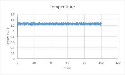
The simulation reaches equilibrium at about t=0.3 and the total energy at equilibrium is about -3.18(in reduced unit).

The pressure and temperature of the system also reach a constant average value with fluctuations, which is 2.6 and 1.3 respectively.

Figure 8: energy versus time for all of the timesteps

Of the five timesteps used, 0.0025 is the largest to give acceptable results. It gives the most similar results as 0.001 timestep. 0.015 is a particularly bad choice because the simulation does not reach an equilibrium and the total energy keeps increasing.

Temperature and Pressure Control

Thermostats and Barostats

In our system with $N$ atoms each with 3 degrees of freedom:

$E_K=\frac{3}{2}N{k}_{B}T$ $\frac{1}{2}\sum _i{m}_i{v}_i^2=\frac{3}{2}N{k}_{B}T$

In order to get our target temperature $\mathfrak{𝔗}$, every velocity can be multiplied by a constant factor $\gamma$:

$\frac{1}{2}\sum _i{m}_i(v_i\gamma {)}^2=\frac{3}{2}N{k}_B\mathfrak{𝔗}$

This equation can be simplified as below:

${\gamma }^2\frac{1}{2}\sum _i{m}_i{v}_i^2=\frac{3}{2}N{k}_B\mathfrak{𝔗}$

${\gamma }^2\frac{3}{2}N{k}_{B}T=\frac{3}{2}N{k}_B\mathfrak{𝔗}$

${\gamma }^{2}T=\mathfrak{𝔗}$

$\gamma =\sqrt{\frac{\mathfrak{𝔗}}{T}}$

Examining the Input Script

fix aves all ave/time 100 1000 100000 v_dens v_temp v_press v_dens2 v_temp2 v_press2
run 100000

The Nevery, Nrepeat, and Nfreq arguments (100, 1000, 10000 in this case) specify on what timesteps the input values will be used in order to contribute to the average. The final averaged quantities are generated on timesteps that are a multiple of Nfreq. The average is over Nrepeat quantities, computed in the preceding portion of the simulation every Nevery timesteps.

The values will be sampled for the average every 100 timesteps and there are 1000 measurements contribute to the average.Then values on timesteps 100, 200, ... 100000 will be used to compute the final average on timestep 100000.

The timestep is 0.0025 and the simulation is run over 100000 timesteps, so the total time of simulation should be 250.

Plotting the Equations of State

10 simulations was run at 5 different temperatures (T=2.0, 3.0, 4.0, 5.0, 6.0) and 2 different pressures (P=2.6, 3.0) at 0.0025 timestep as it shows the best results in last section.

The ideal gas law shows $PV=N{k}_{B}T$, which can be used to calculate density as the equation showing below:

$\rho =\frac{N}{V}=\frac{P}{k_{B}T}$

Since all variables are in reduced units after simulation and $P^{*}=\frac{P{\sigma }^3}{ϵ}$, $\rho =\frac{N{\sigma }^3}{V}$, $T^{*}=\frac{k_{B}T}{ϵ}$ , the density predicted by ideal gas law can be calculated as below:

${\rho }^{*}=\frac{{\sigma }^{3}N}{V}=\frac{{\sigma }^{3}P}{k_{B}T}=\frac{{\sigma }^3\frac{P^{*}ϵ}{{\sigma }^3}}{T^{*}ϵ}=\frac{P^{*}}{T^{*}}$

Figure 9:density vs time for both of the pressures

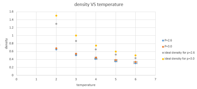
From the graph, it can be seen that the simulated density is lower than the ideal density and the discrepancy increases as pressure increases and it decreases as temperature increases.

Calculating heat capacities using statistical physics

The heat capacity of the system can be calculated by the equation showing below:

$C_V=\frac{\partial E}{\partial T}=\frac{\mathrm{V}\mathrm{a}\mathrm{r}\left[E\right]}{k_B{T}^2}=N^2\frac{⟨E^2⟩-{⟨E⟩}^2}{k_B{T}^2}$

In this case, the temperatures and densities used are 2.0,2.2,2.4,2.6,2.8 and 0.2, 0.8 respectively.

One of the input scripts is shown below:

variable dens equal 0.2
### DEFINE SIMULATION BOX GEOMETRY ###
lattice sc ${dens}
region box block 0 15 0 15 0 15
create_box 1 box
create_atoms 1 box

### DEFINE PHYSICAL PROPERTIES OF ATOMS ###
mass 1 1.0
pair_style lj/cut/opt 3.0
pair_coeff 1 1 1.0 1.0
neighbor 2.0 bin

### SPECIFY THE REQUIRED THERMODYNAMIC STATE ###
variable T equal 2.0
variable timestep equal 0.0025

### ASSIGN ATOMIC VELOCITIES ###
velocity all create ${T} 12345 dist gaussian rot yes mom yes

### SPECIFY ENSEMBLE ###
timestep ${timestep}
fix nve all nve

### THERMODYNAMIC OUTPUT CONTROL ###
thermo_style custom time etotal temp press
thermo 10

### RECORD TRAJECTORY ###
dump traj all custom 1000 output-1 id x y z

### SPECIFY TIMESTEP ###

### RUN SIMULATION TO MELT CRYSTAL ###
run 10000
unfix nve
reset_timestep 0

### BRING SYSTEM TO REQUIRED STATE ###
variable tdamp equal ${timestep}*100
fix nvt all nvt temp ${T} ${T} ${tdamp} 
run 10000
reset_timestep 0

### MEASURE SYSTEM STATE ###
thermo_style custom step etotal temp vol atoms
variable volume equal vol
variable atoms2 equal atoms*atoms
variable temp equal temp
variable temp2 equal temp*temp
variable E equal etotal
variable E2 equal etotal*etotal
fix aves all ave/time 100 1000 100000 v_temp v_temp2 v_volume v_E v_E2
unfix nvt
fix nve all nve
run 100000

variable avetemp equal f_aves[1]
variable heatcapacity equal ${atoms2}*(f_aves[5]-f_aves[4]*f_aves[4])/f_aves[2]
variable heatcapacityV equal ${heatcapacity}/${volume}

print "Averages"
print "--------"
print "Temperature: ${avetemp}"
print "Heat Capacity: ${heatcapacity}"
print "Heat Capacity over V: ${heatcapacityV}"

In order to make the heat capacity independent of the size, we plot $\frac{C_v}{V}$ against temperature.

figure 10: Cv/V against temperature for two different densities

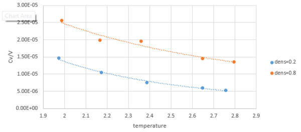
According to the equation, the temperature and heat capacity are inversely proportional. So the value of $\frac{C_v}{V}$ should decrease with temperature.

As for a larger density system, it will have more atoms at a fixed volume and the ability of it to store internal energy will be stronger, therefore the value of $\frac{C_v}{V}$ at $\rho =0.8$ will be higher than at$\rho =0.2$.

Structural properties and the radial distribution function

An atomic trajectory is recorded to generate RDFs for the solid, liquid, and vapour phase Lennard Jones systems. In order to get 3 different phases, the density and temperature is modified as below :

	vapour	liquid	solid
Temperature	1.15	1.2	1.15
Density	0.05	0.8	1.5

Figure 11: RDFs for 3 systems

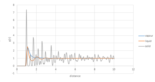
The RDF[1] defines the probability of finding a particle at a distance r from another particle. For all 3 systems, when r is small, the value of g(r) is zero as two particles can not occupy the same space due to repulsion forces and the first coordination sphere is found when $r=\sigma$.

Gases do not have a regular structure and only have one coordination sphere that will rapidly decay to normal density, g(r)=1.

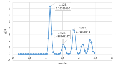
Solids have regular and specific structure over a long range. The peaks indicate the coordination shells for the solid. The first peak represents the nearest neighbours, the second peaks is for the second nearest neighbours and so on. There is no possibility to find particles in between as all molecules are regularly packed.

Liquids are more loosely packed than solids, therefore, do not have exact intervals.

Figure 12:first 3 peaks in RDF of solid

Figure 13: running integral of RDF of solid

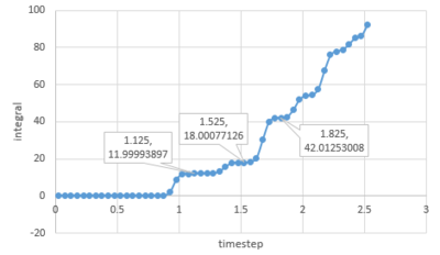Acoording to the plot above, as for solid, the coordination number of the first coordination shell is 12. And the coordination number for the second and third shell is 6 and 24 respectively.

Dynamical properties and the diffusion coefficient

Mean Squared Displacement

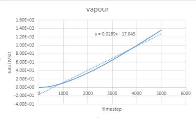
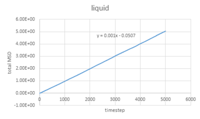
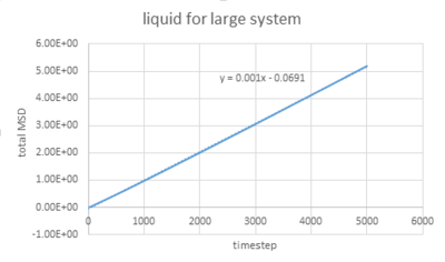
The densities and temperatures used are the same as last section. The graphs below show the simulation of MSD of liquid, solid and gas as well as for a 1 million atoms system.

Figure 14a: Simulation for gas

Figure 14b: simulation for liquid

Figure 14c:simulation for solid

Figure 15a: Simulation for gas (much larger system)

Figure 15b: simulation for liquid (much larger system)

Figure 15c: Simulation for solid (much larger system)

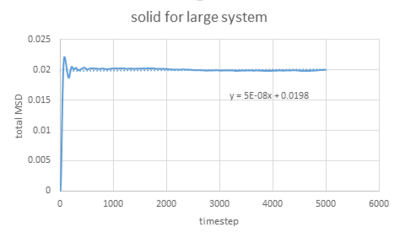The graphs vapour and liquid for both small and large scales are nearly the same. The graph for solid at a small scale looks similar to the larger system one but with more fluctuations because the stability of a system containing 1 million atoms would be much higher.

Solid shows a completely different shape due to its regular structure and it has a fixed position for each atom (with vibrations).

The value of D can be estimated by the equation showing below:

$D=\frac{1}{6}\frac{\partial ⟨r^2\left(t\right)⟩}{\partial t}$

In this case, $\frac{\partial ⟨r^2\left(t\right)⟩}{\partial t}$=gradient of trend line /timestep.

As for small systems,

vapour: $D=\frac{1}{6}\times \frac{0.0289}{0.002}=2.408$

liquid: $D=\frac{1}{6}\times \frac{0.001}{0.002}=0.083$

solid: $D=\frac{1}{6}\times \frac{6\times 10^{-9}}{0.002}=5\times 10^{-7}$

As for larger systems,

vapour: $D=\frac{1}{6}\times \frac{0.0305}{0.002}=2.542$

liquid: $D=\frac{1}{6}\times \frac{0.001}{0.002}=0.083$

solid: $D=\frac{1}{6}\times \frac{5\times 10^{-8}}{0.002}=4.17\times 10^{-6}$

Velocity Autocorrelation Function

The equation for the evolution of the position of a 1D harmonic oscillator as a function of time is shown below:

$x(t)=Acos(\omega t+\varphi )$

Since $v(t)=\frac{dx(t)}{dt}$,

$v(t)=\frac{d[Acos(\omega t+\varphi )]}{dt}=-\omega Asin(\omega t+\varphi )$

$v(t+\tau )=-\omega Asin[\omega (t+\tau )+\varphi =-\omega Asin[\omega (t+\varphi )+\omega \tau ]$

Acoording to the trigonometric formula $sin(x+y)=sin(x)cos(y)+cos(x)sin(y)$:

$v(t+\tau )=-\omega A[sin(\omega t+\varphi )cos(\omega \tau )+cos(\omega t+\varphi )sin(\omega \tau )]=cos(\omega \tau )\times v(t)-\omega t[cos(\omega t+\varphi )sin(\omega \tau )]$

Since $C\left(\tau \right)=\frac{\underset{-\mathrm{\infty }}{\overset{\mathrm{\infty }}{\int }}v\left(t\right)v(t+\tau )\mathrm{d}t}{\underset{-\mathrm{\infty }}{\overset{\mathrm{\infty }}{\int }}{v}^2\left(t\right)\mathrm{d}t}$,

$C(\tau )=\frac{\underset{-\mathrm{\infty }}{\overset{\mathrm{\infty }}{\int }}v(t)[v(t)cos(\omega \tau )-\omega t[cos(\omega t+\varphi )sin(\omega \tau )]]\mathrm{d}t}{\underset{-\mathrm{\infty }}{\overset{\mathrm{\infty }}{\int }}{v}^2(t)\mathrm{d}t}$

$C(\tau )=\frac{cos(\omega t)\underset{-\mathrm{\infty }}{\overset{\mathrm{\infty }}{\int }}{v}^2(t)\mathrm{d}t}{\underset{-\mathrm{\infty }}{\overset{\mathrm{\infty }}{\int }}{v}^2(t)\mathrm{d}t}-\frac{\underset{-\mathrm{\infty }}{\overset{\mathrm{\infty }}{\int }}-\omega t[cos(\omega t+\varphi )sin(\omega \tau )]\mathrm{d}t}{\underset{-\mathrm{\infty }}{\overset{\mathrm{\infty }}{\int }}{v}^2(t)\mathrm{d}t}$

$C(\tau )=cos(\omega t)-\frac{\underset{-\mathrm{\infty }}{\overset{\mathrm{\infty }}{\int }}-\omega t[cos(\omega t+\varphi )sin(\omega \tau )]\mathrm{d}t}{\underset{-\mathrm{\infty }}{\overset{\mathrm{\infty }}{\int }}{v}^2(t)\mathrm{d}t}$

Sine function is an odd function, which means the integral of it from $-\mathrm{\infty }$ to $\mathrm{\infty }$ will be zero. Therefore the second part of the equation shown above should also be zero.

Then the equation can be simplified to:

$C(\tau )=cos(\omega \tau )$

The graph below shows the difference between VACFs of Lennard Jones liquid and solid and harmonic oscillator VACF.

Figure 16: VACFs for liquid, solid and $\omega =\frac{1}{2\pi }$

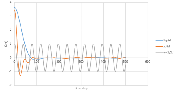
The velocity of a molecule after the collision will be independent of its initial velocity. Both magnitude and direction are expected to change with the influence of the force. The minimum value on the graph corresponds to the largest difference between final velocity and initial velocity. Solid has a lower value than the liquid due to stronger interatomic force. In the case of harmonic oscillator, the interatomic force is not involved.

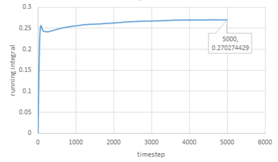
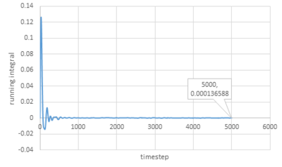
The following equation can be used to calculate D:

$D=\frac{1}{3}\underset{0}{\overset{\mathrm{\infty }}{\int }}\mathrm{d}\tau ⟨\mathbf{v}\left(0\right)\cdot \mathbf{v}\left(\tau \right)⟩$

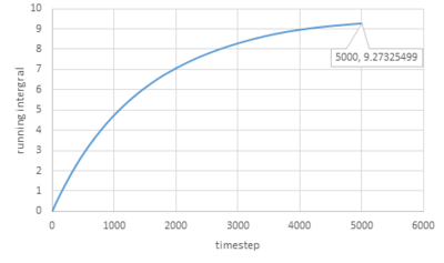
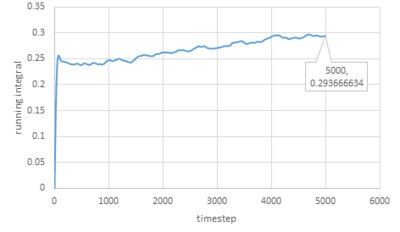
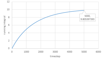
Trapezium rule is then used to estimate the integrals under VACFs for gas, liquid and solid and the plots of running integral are shown below:

Figure 17a: running integral for gas

Figure 17b: running integral for liquid

Figure 17c: running integral for solid

As for larger systems:

Figure 18a: running integral for gas

Figure 18b: running integral for liquid

Figure 18c: running integral for solid

Calculations for values of D for small systems:

gas: $D=\frac{1}{3}\times 9.27325499=3.091$

liquid: $D=\frac{1}{3}\times 0.293666634=0.098$

solid: $D=\frac{1}{3}\times 0.002980073=9.933\times 10^{-4}$

As for larger systems:

gas: $D=\frac{1}{3}\times 9.805397393=3.268$

liquid: $D=\frac{1}{3}\times 0.270274429=0.090$

solid: $D=\frac{1}{3}\times 0.000136588=4.553\times 10^{-5}$

The values of D obtained are very close to the values from the last section except for the value of solid.

The trapezium rule is not that accurate especially for solid and it can be improved by smaller timestep.

References

- ↑ S. Delage Santacreu ,G. Galliero, M. Odunlami and C. Boned, "Low density shear viscosity of Lennard-Jones chains of variable rigidities", J. Chem. Phys., 137, 204306(2012). DOI:10.1063/1.4767528
- ↑ Jean-Pierre Hansen and Loup Verlet, "Phase Transitions of the Lennard-Jones System", Phys. Rev., 184, 151, 1969.DOI:10.1103/PhysRev.184.151
- ↑ Otto J. Eder, "The velocity autocorrelation function and the diffusion coefficient for a dilute hard sphere gas", J. Chem. Phys., 66, 3866 (1977).DOI:10.1063/1.434461