
Rep:Mod:xl3209module2
Third Year Computational Project: Module 2, Xizhou Liu, CID: 00593697
-Inorganic Computational Project
Introduction
In module 1, the computational analysis was focused on the Organic Chemistry mainly. Since the reactive intermediates are one of the key research areas, predicting 13C NMR spectra and IR spectra allows to rationalize the structure of the reactive intermediates, i.e. the conformational analysis, isomerization analysis, kinetic effects vs thermodynamic effects.
However the computational analysis is extended further to the scope of Inorganic Chemistry in this module. The main focus here is the nature of the bonds formed between atoms. Vibrational analysis, molecular orbitals and natural bond orbitals analysis generated by Gaussian allows to rationalize the nature of the bonds (i.e to draw analogies between BH3 and TlBr3 molecules, determine the difference in the cis and tran Mo(CO)4Cl2 complex, and finally explain the variations in higher hapticity ηn complexes). Therefore computational analysis has the ability to assist chemists in exploring new chemical bonding nature. It has many advantages compared to standard laboratory experiments (i.e. reducing reagent costs, avoidance issues as toxicity). By comparing the computational outcomes to literature values, it is possible to understand the degree of accuracy of the computational analysis. This is really important as computational analysis is not useful in understanding chemical natures if the method used is not reliable.
The definition of optimization: Optimization is the first stage at every computational analysis. In order to obtain any useful calculations, the optimization must be performed and performed correctly. In this experiment, the optimization can be defined in two parts:
- SCF part: The position of the nuclei (i.e. boron and hydrogen) are defined manually by the known knowledge of the molecules. This allows the electron density and the energy to be solved via the Schrödinger equation.
- OPT part: The position of the nuclei are moved and the SCF cycles are repeated at each new geometry. The final geometry reported is the geometry with the lowest energy in the cycles.
Accuracy: Accuracy plays an important role in every analysis, the degree of accuracy can be analyzed if compare with literature.
- Energy:
The energy will normally have an error of ca. 10 KJmol-1. Since 1 Ha = 4.359744 x 10⁻¹⁸ J (equivalent to ca.2625 KJmol-1, the energy reported in Hartree (a.u. unit) should have the an error of ca. 0.004 a.u.. Therefore the energies are considered only to the nearest 0.01 a.u..
- Dipole Moment
The dipole moment are accurate to ca. 2 decimal places and considered to the nearest 0.01 Deby.
- Frequencies
Because the harmonic approximation approach used in the following calculations, there is a ca. 10% systematic error induced due to the anharmonic nature. i.e. for vibrations in the order of 1000 cm-1, the vibration energy error is ca. 100 cm-1. However, by convention, the frequencies are reported to the nearest integer number.
- Intensities
The intensities are rounded conventionally to the nearest integer number.
- Bond distances
They are rounded to the nearest 0.01 Å.
- Bond angles
They are considered to the nearest 0.1°.
BH3
Optimisation of Geometry
The BH3 bonds was set to 1.50 Å in Gauss view. The optimised structure is attached . The optimised bond distance is 1.19 Å and bond angle is 120.0o.
Commands of calculations:
- The method (type of approximations in Schrödinger equation): DFT/B3LYP
- The basis set (the accuracy of the calculation): 3-21G
- Type of calculation: OPT
The Results of Optimisation (BH3 Log file [1])
| Table 1. BH3 Optimisation Summary | BH3 Optimisation Parameter |
|
File Name = bh3_optimisation Charge = 0 Spin = Singlet E(RB3LYP) = -26.46 a.u. RMS Gradient Norm = 0.00 a.u. Imaginary Freq =0 Dipole Moment = 0.00 Debye Point Group = D3H |
 |
Note: it is important to check the log file after each optimization performed to confirm that the items listed are converged as shown in Table 1. The optimized parameter listed above also gives information on the structure of the BH3 molecule.
Optimisation Progress
As illustrated in total energy and RMS gradient Norm (Figure 1), the optimisation of the B-H bond lengths takes four steps in the progress from 1.5 Å to 1.19 Å. A gradual decrease in total energy is observed and Gauss shows no bond formation until step 3. Since the Gauss view can only recognize bond formation within certain distances.

Vibrational Analysis
The vibrational analysis are first carried out using the B3LYP method with a small basis set 3-21G. The frequencies observed are listed in Table 2 BH3 Frequency Profile below. The top line of the low frequencies represent the "-6" vibrational modes (every molecule has 3N-6 vibrational frequencies). In other words, these -6 vibrational frequencies are the motions caused by the center of the mass of the molecule. These values should be much smaller than the first vibration listed (1144 cm -1), for example the largest "zero" energy should be ca. 40 cm-1. However the negative frequencies are listed to be around 66 cm-1, which is larger than expected. As suggested, improving the basis sets employed may result in bringing the "zero" energies closer to be within +/- -10 cm-1. Therefore the second calculation is performed by keeping the same B3LYP method, but changing the basis set from 3-21G to 6-31G(d,p). The results are included below to compare.
Commands of calculations (3-21G)
- The method (type of approximations in Schrödinger equation): B3LYP
- The basis set (the accuracy of the calculation): 3-21G
- Type of calculation: FREQ
- Additional key word: pop=(full,nbo)
Results of vibrational calculation (3-21G) BH3 Frequency (3-21G) Log file[2]
Charge = 0 Spin = Singlet E(RB3LYP) = -26.46 a.u. RMS Gradient Norm = 0.00 a.u. Imaginary Freq =0 Dipole Moment = 0.00 Debye Point Group = C3H |
 |
It is worth to note that Gaussian has a bug here as giving a different point group of the frequency analysis log file of the BH3 molecule compare to the optimization log file. However by improving the basis set, this contradiction disappears.
Commands of calculations (6-31G(d,p)):
- The method (type of approximations in Schrödinger equation): B3LYP
- The basis set (the accuracy of the calculation): 6-31G(d,p)
- Type of calculation: FREQ
- Additional key word: pop=(full,nbo)
Results of vibrational calculation (6-31G(d,p)) BH3 Frequency (6-31G(d,p)) Log file[3]
Charge = 0 Spin = Singlet E(RB3LYP) = -26.32 a.u. RMS Gradient Norm = 0.00 a.u. Imaginary Freq =0 Dipole Moment = 0.00 Debye Point Group = D3H |
 |
By comparing the Table 2 and Table 3, a significant contrast (decrease in a order of magnitude of 5) in the "zero" vibrational frequencies can be seen by changing to the 6-31G(d,p) basis set. Therefore this brings the "zero" energy closer to minimum. By doing so, the vibrational frequencies can be predicted more accurately. Thus, further analysis is carried on the 6-31G(d,p) basis set method.
IR spectrum of BH3 molecule (6-31G(d,p))
The IR spectrum of BH3 molecule is in Figure 2 and the log file[4] in the reference.

| Entry | Type | Animation | Mode | Vibrational Annotation | Frequency/ cm-1 | Lit./ cm-1 [5] | Intensity | Symmetry |
|---|---|---|---|---|---|---|---|---|
| 1 | Wagging |  |
 |
All hydrogen atoms move up and down the plane in a concerted manner, while the boron atom moves up and down in an opposite direction. There is a large change in dipole moment. Hence the intensity is strong. | 1163 | 1225 | 93 | A2" |
| 2 | Scissoring |  |
 |
Two hydrogen atoms move closer and further to each other in a concerted manner, while the other hydrogen atom and boron atom displace slightly from the plane of the two hydrogen atoms. There is very small change of dipole moment. Hence the vibrational mode is weak. | 1213a | 1305 | 14 | E' |
| 3 | Rocking |  |
 |
Two hydrogen atoms move closer and further to each other as the scissoring mode, while the other hydrogen atom moves across the plane perpendicular to the plane of the two hydrogen atoms. There is very small change of dipole moment. Hence the vibrational mode is weak. | 1213b | 1305 | 14 | E' |
| 4 | Symmetric Stretching |  |
 |
All hydrogen atoms move in and out together in a concerted manner, while the boron atom remains stationary. There is absent of change of dipole moment. Hence the vibrational mode has zero intensity and cannot be observed in the spectrum. | 2582 | not observed as no intensity | 0 | A1' |
| 5 | Asymmetric Stretching |  |
 |
Two hydrogen atoms stretch in a non-concerted manner, while the other hydrogen atom and boron atom remain still. There is very large change of dipole moment. Hence the vibrational mode is very strong. | 2715a | 2693 | 126 | E' |
| 6 | Asymmetric Stretching |  |
 |
Two hydrogen atoms stretch in a concerted manner, while the other hydrogen atom stretches in the opposite direction. The boron atom remains still. There is very large change of dipole moment. Hence the vibrational mode is very strong. | 2715b | 2693 | 126 | E' |
As shown in Figure 2, only 3 vibrational frequencies are observed in the IR Spectrum, whilst in principle should be 6 vibrational modes according to 3N-6 rule. This can be explained in terms of the vibrational frequencies and their corresponding intensities. By inspection, the "disappeared" A1' all symmetrical stretch frequency has zero intensity. This is because the lack of change in dipole moment. As the vibrational modes can only be observed in IR spectrum if they have a change in dipole moment. Furthermore, the two sets of degenerate E' vibrational stretches are present and they only contribute to two peaks in the spectrum as the overlap effect.
The vibrational frequencies are compared to literature frequencies, as expected, these values agree to the literature values.
Molecular Orbitals
The predicted molecular orbital of BH3 was constructed as following:[6]
- Determine the shape of the molecule using VSEPR model & identify the point group of the molecular:
Trigonal planar, D3h
- Define the axial system: choose the z-axis to be the highest rotational axis, and therefore the Bh3 molecule is in the plane of the xy
- List all the symmetry elements(as shown in Figure 3)
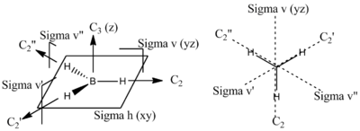
Figure 3 BH3 Axial System and Symmetry Elements

- Identify the fragments: in this case, the B atom and H3 fragment
- Determine the energy levels and symmetry labels of the fragment orbital:
Totally bonding fragment orbitals of H3 are totally symmetric and thus have a1' symmmetry Degenerate fragment orbitals of H3 have either e' or e" symmetry The orbitals of the boron atom must be determined by the symmetry labels of the x, y, z axes. (px, py atomic orbitals are degenerate and thus have e' symmetry, pz atomic orbital has a2" symmetry and s atomic orbitals are always totally symmetric and thus have a1' symmetry)
- Estimate the relative positions of the energies of the fragment orbitals:
Since boron and hydrogen atoms are all electropositive elements and therefore their s AOs start at approximately the same level. (the H3 fragment bonding orbitals are slightly lower in energy because the stablising interactions between the in-phase three s AOs). The H3 fragment anti-bonding orbitals are slightly higher in energy than the boron 2s AO, because the destablising interactions are again small since the hydrogen orbitals are not close enough to have a strong effect.
- Combine the orbitals with the same symmetry and estimate the bonding/anti-bonding character and the extent of energy splitting
The molecular orbitals generated by prediction of the method of Linear Combination of Atomic Orbitals and calculations in Gaussian are listed below in Table 5 for comparison.
| LCAO MO diagram predicted by theory | MO diagram calculated by Gaussian [7] | MO Annotation | Molecular Orbital | |
|---|---|---|---|---|
 | ||||
 |
3a1' higher than 2e', possibly because s-s interactions are stronger than s-p interactions | LUMO+3 | ||
 |
out-of-phase overlap, strong anti-bonding MO | LUMO+2 | ||
 |
out-of-phase overlap, strong anti-bonding MO | LUMO+1 | ||
 |
a2" boron orbital, non-bonding MO | LUMO | ||
 |
e' fragment orbitals, in-phase overlap, bonding interactions are large. | HOMO | ||
 |
e' fragment orbitals, in-phase overlap, bonding interactions are large. | HOMO-1 | ||
 |
low energy a1' fragment orbitals, in-phase overlap, bonding interactions are very large. | HOMO-2 | ||
 |
low lying boron AO, not involved in bonding | HOMO-3 |
Conclusion:
- In general, it can be seen that from HOMO-3 to LUMO+3 obtained by Gaussian, more nodal planes appear in the MOs, larger anti-bonding interactions.
- The detailed annotations of each molecular orbital are included in table 5,
- It is worth to mention that 3a1' MO is higher in energy than 2e' MO. As explained in Table 5 This is probably because s-s interactions are stronger than s-p interactions in the DFT/B3LYP method and 6-31G(d,p) basis set used. In reality this mixing contribution is hard to rationalize as changing the methods and basis sets may result in different energies.
- As seen from the table, the theory and the calculation agree to each other, which indicates that the LCAO approach to the molecular orbital analysis for small molecules i.e BH3 is successful. The LCAO theory is said to be sufficient to analyze the nature of bonding of these small molecules as the variations to quantum mechanical calculations are small.
NBO Analysis
The same log file used as the MO analysis.[8]
Natural bond orbital (NBO) analysis is a method optimally transforming wave functions of atoms in a molecule into localised form, (referring to the one centre lone pairs and two centre bonds of the lewis structure picture).
The full NBO analysis of BH3 molecule is obtained in Gaussian by adding the additional key word: pop=(full,nbo). Table 6 below is the numerical summary of the natural population analysis (NPA). The table describes the molecular charge distribution in terms of the NPA charges. The boron atom of the BH3 molecule, for example, is assigned a net NPA charge of +0.30 at this level. The three hydrogen atoms are assigned net negative charges of -0.10.
Table 6. Summary of Natural Population Analysis:

                                      Natural Population
               Natural  -----------------------------------------------
   Atom  No    Charge         Core      Valence    Rydberg      Total
-----------------------------------------------------------------------
     B    1    0.29733      1.99964     2.70037    0.00266     4.70267
     H    2   -0.09911      0.00000     1.09852    0.00059     1.09911
     H    3   -0.09911      0.00000     1.09852    0.00059     1.09911
     H    4   -0.09911      0.00000     1.09852    0.00059     1.09911
=======================================================================
  * Total *    0.00000      1.99964     5.99594    0.00442     8.00000
|
Below is just the pictorial representation of the natural population analysis:
| Figure 4 BH3 NBO Charge Distributions by color | Figure 5 BH3 NBO Charge Distributions by number |
 |
 |
Moving down the log file, the natural populations can be further interpreted as natural electron configuration (effective valence electron configuration) for each atom in the molecule. From table 7, it can be seen that the natural electron configurations are non-integer numbers and these non-integer numbers can be related to idealised situations but in promoted configurations. For example, the boron atom below can be described as 1s22s0.982p1.72 electronic configuration (idealised bond sp2).
Table 7. Natural Electron Configuration Atom No Natural Electron Configuration
----------------------------------------------------------------------------
B 1 [core]2S( 0.98)2p( 1.72)
H 2 1S( 1.10)
H 3 1S( 1.10)
H 4 1S( 1.10)
|
Further down the log file, the output that summarizes the results of the NBO analysis can be obtained in table 8. The first segment gives a detailed search for the NBO natural lewis structure. The cycle is normally a single cycle. The properties in the table represent the following: the occupancy threshold for a good pair in the NBO search (Thresh); the population of Lewis and non-Lewis orbitals; the number of core (CR); 2-centre bond (BD); 3-centre bond (3C); lone pair (LP); the number of the Lewis orbitals (low-occupancy, L) and non-Lewis orbitals (high-occupancy, NL); and the maximum deviation of any formal bond order from the estimate structure (Dev). This is then followed by a detailed breakdown of the Lewis and non-Lewis occupancies into core, valence and Rydberg shell contributions. The total Lewis percentage is reported as exceeding 99.9%, which means the quality of the natural Lewis description in terms of the total electron density is good.
Table 8. NATURAL BOND ORBITAL ANALYSIS: Occupancies Lewis Structure Low High
Occ. ------------------- ----------------- occ occ
Cycle Thresh. Lewis Non-Lewis CR BD 3C LP (L) (NL) Dev
=============================================================================
1(1) 1.90 7.99444 0.00556 1 3 0 0 0 0 0.00
-----------------------------------------------------------------------------
Structure accepted: No low occupancy Lewis orbitals -------------------------------------------------------- Core 1.99964 ( 99.982% of 2) Valence Lewis 5.99480 ( 99.913% of 6) ================== ============================ Total Lewis 7.99444 ( 99.930% of 8) ----------------------------------------------------- Valence non-Lewis 0.00514 ( 0.064% of 8) Rydberg non-Lewis 0.00042 ( 0.005% of 8) ================== ============================ Total non-Lewis 0.00556 ( 0.070% of 8) -------------------------------------------------------- |
"Bond orbital coefficients/ hybrids" is listed in table 9, this describes the bonding in the molecule. (Only the key informations are shown here)
- The first bond (BD) is between boron (atom 1) and hydrogen (atom 2) and 45% of the bond is contributed from the boron orbitals (with hybridisation of 33% s character + 67% p character). The other 55% of the bond is contributed from the hydrogen orbital (with hybridisation of 100% s character).
- The second and third bonds are the same as the first boron and hydrogen bond.
- Overall the boron and three hydrogen atoms form three bonds (best described as interactions between 3 sp2 hybrid orbitals of B with s AOs of H atoms.
- Orbital 4 is the core 1s AO of boron.
Table 9.        (Occupancy)   Bond orbital/ Coefficients/ Hybrids
---------------------------------------------------------------------------------
    1. (1.99827) BD ( 1) B   1 - H   2
               ( 45.04%)   0.6711* B   1 s( 33.31%)p 2.00( 66.59%)d 0.00(  0.10%)
                                           0.0000  0.5772  0.0000  0.0000  0.0000
                                           0.0000  0.8160  0.0000  0.0000  0.0000
                                           0.0000  0.0000  0.0000 -0.0282 -0.0142
               ( 54.96%)   0.7413* H   2 s( 99.96%)p 0.00(  0.04%)
                                           0.9998 -0.0001  0.0000 -0.0202  0.0000
    2. (1.99827) BD ( 1) B   1 - H   3
               ( 45.04%)   0.6711* B   1 s( 33.31%)p 2.00( 66.59%)d 0.00(  0.10%)
                                           0.0000  0.5772  0.0000  0.0000 -0.7067
                                           0.0000 -0.4080  0.0000  0.0000  0.0000
                                           0.0245  0.0000  0.0000  0.0141 -0.0142
               ( 54.96%)   0.7413* H   3 s( 99.96%)p 0.00(  0.04%)
                                           0.9998 -0.0001  0.0175  0.0101  0.0000
    3. (1.99827) BD ( 1) B   1 - H   4
               ( 45.04%)   0.6711* B   1 s( 33.31%)p 2.00( 66.59%)d 0.00(  0.10%)
                                           0.0000  0.5772  0.0000  0.0000  0.7067
                                           0.0000 -0.4080  0.0000  0.0000  0.0000
                                          -0.0245  0.0000  0.0000  0.0141 -0.0142
               ( 54.96%)   0.7413* H   4 s( 99.96%)p 0.00(  0.04%)
                                           0.9998 -0.0001 -0.0175  0.0101  0.0000
    4. (1.99964) CR ( 1) B   1           s(100.00%)
                                           1.0000  0.0000  0.0000  0.0000  0.0000
                                           0.0000  0.0000  0.0000  0.0000  0.0000
                                           0.0000  0.0000  0.0000  0.0000  0.0000
    5. (0.00000) LP*( 1) B   1           s(100.00%)
|
"Second order perturbation theory analysis" is reported in table 10, this includes mainly the interactions between bonding and antibonding NBOs. All the E2 energies are ca. 0.5 kcal/mol, which means the interactions are weak. Therefore the mixing between the NBOs are not particular strong for BH3 here.
Table 10.
Second Order Perturbation Theory Analysis of Fock Matrix in NBO Basis Threshold for printing: 0.50 kcal/mol
E(2) E(j)-E(i) F(i,j)
Donor NBO (i) Acceptor NBO (j) kcal/mol a.u. a.u.
===================================================================================================
within unit 1 1. BD ( 1) B 1 - H 2 / 29. BD*( 1) B 1 - H 3 0.55 0.87 0.020 1. BD ( 1) B 1 - H 2 / 30. BD*( 1) B 1 - H 4 0.55 0.87 0.020 2. BD ( 1) B 1 - H 3 / 28. BD*( 1) B 1 - H 2 0.55 0.87 0.020 2. BD ( 1) B 1 - H 3 / 30. BD*( 1) B 1 - H 4 0.55 0.87 0.020 3. BD ( 1) B 1 - H 4 / 28. BD*( 1) B 1 - H 2 0.55 0.87 0.020 3. BD ( 1) B 1 - H 4 / 29. BD*( 1) B 1 - H 3 0.55 0.87 0.020 4. CR ( 1) B 1 / 16. RY*( 1) H 2 0.57 7.45 0.058 4. CR ( 1) B 1 / 20. RY*( 1) H 3 0.57 7.45 0.058 4. CR ( 1) B 1 / 24. RY*( 1) H 4 0.57 7.45 0.058 |
Finally, the summary of the NBOs are shown in table 11, showing the occupancy, energy and etc. It is worth to noted the three bonding interactions and 1s core AO for boron atom.
Table 11.
Natural Bond Orbitals (Summary): Principal Delocalizations
NBO Occupancy Energy (geminal,vicinal,remote)
====================================================================================
Molecular unit 1 (H3B)
1. BD ( 1) B 1 - H 2 1.99827 -0.43089 29(g),30(g)
2. BD ( 1) B 1 - H 3 1.99827 -0.43089 28(g),30(g)
3. BD ( 1) B 1 - H 4 1.99827 -0.43089 28(g),29(g)
4. CR ( 1) B 1 1.99964 -6.68893 16(v),20(v),24(v)
5. LP*( 1) B 1 0.00000 0.54800
|
TlBrs
Optimisation of Geometry
The TlBr3 optimisation is performed just as the BH3 molecule. LanL2DZ basis set is used here instead of the 3-21G basis set used before. LanL2DZ uses a medium level basis set: D95V on first row atoms and Los Alamos ECP (effective core potential) on heavier elements. Thallium and bromine are heavy atoms that cannot be recovered by the standard Schrodinger equation due to relativistic effects. Therefore using pseudo-potential makes calculations of heavier elements much easier and faster. The optimised structure is attached . The optimised bond distance is 2.65 Å and bond angle is 120.0o.
Commands of calculations:
- The method (type of approximations in Schrödinger equation): B3LYP
- The basis set (the accuracy of the calculation): LanL2DZ
- Type of calculation: OPT
The Results of Optimisation
TlBr3 OptimisationLog file[9]
| Table 12. TlBr3 Optimisation Summary | TlBr3 Optimisation Parameter |
| File Name = tlbr3_optimisation
Charge = 0 Spin = Singlet E(RB3LYP) = -91.22 a.u. RMS Gradient Norm = 0.00 a.u. Imaginary Freq =0 Dipole Moment = 0.00 Debye Point Group = D3H |
        Item               Value     Threshold  Converged?
Maximum Force            0.000002     0.000450     YES
RMS     Force            0.000001     0.000300     YES
Maximum Displacement     0.000022     0.001800     YES
RMS     Displacement     0.000014     0.001200     YES
Predicted change in Energy=-6.083939D-11
Optimization completed.
   -- Stationary point found.
                          ----------------------------
                             Optimized Parameters
                           (Angstroms and Degrees)
--------------------------                            --------------------------
 Name  Definition              Value          Derivative Info.
--------------------------------------------------------------------------------
 R1    R(1,2)                  2.651          -DE/DX =    0.0
 R2    R(1,3)                  2.651          -DE/DX =    0.0
 R3    R(1,4)                  2.651          -DE/DX =    0.0
 A1    A(2,1,3)              120.0            -DE/DX =    0.0
 A2    A(2,1,4)              120.0            -DE/DX =    0.0
 A3    A(3,1,4)              120.0            -DE/DX =    0.0
 D1    D(2,1,4,3)            180.0            -DE/DX =    0.0
--------------------------------------------------------------------------------
|
Again all the items are converged and RMS gradient Norm is ca. 0.00. These indicates the optimization is performed.
Optimisation Progress
As illustrated in total energy and RMS gradient plot (Figure 6) the optimization process takes three iterations and the gradient goes to zero eventually.

Vibrational Analysis
TlBr3 vibrational analysis log file[10]
The vibrational modes are calculated in a same basis set as the optimization. The frequencies observed (as shown below) are reasonable. Since the top line of the low frequencies represent the "-6" vibrational frequencies (every molecule has 3N-6 vibrational frequencies), these are the motions caused by the center of the mass of the molecule. Therefore these values should be much smaller than the first vibration listed (ca. 50 cm -1), the largest "zero" energy should be ca. 0.5 cm-1. The top line shows larger negative frequencies around 4 cm-1. This is ok since only slightly larger than expected. Furthermore, the LanL2DZ basis set used here is a compromise of time and accuracy. It is reasonable result given that the basis set is only medium size.
Commands of calculations
- The method (type of approximations in Schrödinger equation): B3LYP
- The basis set (the accuracy of the calculation): Lan2LDZ
- Type of calculation: FREQ
- Additional key word: pop=(full,nbo)
Results of vibrational calculation
Charge = 0 Spin = Singlet E(RB3LYP) = -91.22 a.u. RMS Gradient Norm = 0.00 a.u. Imaginary Freq =0 Dipole Moment = 0.00 Debye Point Group = D3H |
Low frequencies ---   -3.4213   -0.0026   -0.0004    0.0015    3.9367    3.9367
Low frequencies ---   46.4289   46.4292   52.1449
                    1                      2                      3
                   E'                     E'                     A2"
Frequencies --    46.4289                46.4292                52.1449
Red. masses --    88.4613                88.4613               117.7209
Frc consts  --     0.1124                 0.1124                 0.1886
IR Inten    --     3.6867                 3.6867                 5.8466
 Atom  AN      X      Y      Z        X      Y      Z        X      Y      Z
    1  81     0.00   0.28   0.00    -0.28   0.00   0.00     0.00   0.00   0.55
    2  35     0.00   0.26   0.00     0.74   0.00   0.00     0.00   0.00  -0.48
    3  35     0.43  -0.49   0.00    -0.01  -0.43   0.00     0.00   0.00  -0.48
    4  35    -0.43  -0.49   0.00    -0.01   0.43   0.00     0.00   0.00  -0.48
                    4                      5                      6
                   A1'                    E'                     E'
Frequencies --   165.2685               210.6948               210.6948
Red. masses --    78.9183               101.4032               101.4032
Frc consts  --     1.2700                 2.6522                 2.6522
IR Inten    --     0.0000                25.4830                25.4797
 Atom  AN      X      Y      Z        X      Y      Z        X      Y      Z
    1  81     0.00   0.00   0.00     0.42   0.00   0.00     0.00   0.42   0.00
    2  35     0.00  -0.58   0.00     0.01   0.00   0.00     0.00  -0.74   0.00
    3  35     0.50   0.29   0.00    -0.55  -0.32   0.00    -0.32  -0.18   0.00
    4  35    -0.50   0.29   0.00    -0.55   0.32   0.00     0.32  -0.18   0.00
|

| Entry | Type | Animation | Mode | Vibrational Annotation | Freq./ cm-1 | Lit./ cm-1 [12] | Intensity | Symmetry |
|---|---|---|---|---|---|---|---|---|
| 1 | Scissoring | Link to Animation |  |
Two of the Br atoms move towards each other, while the Tl atom and the remaining Br atom are slightly displaced. moves up and down in an opposite direction. There is a very small change in dipole moment. Hence the intensity is very weak. | 46a | 47 | 4 | E' |
| 2 | Rocking | Link to Animation |  |
Three Br atoms move closer and further to each other in a concerted manner, while the Tl atom remains almost stationary. There is a very small change of dipole moment. Hence the vibrational mode is very weak. | 46b | 47 | 4 | E' |
| 3 | Wagging | Link to Animation |  |
All three of the Br atoms move up and down in the z-axis, while the Tl atom moves in the opposite direction. There is very small change of dipole moment. Hence the vibrational mode is very weak. | 52 | 63 | 6 | A2" |
| 4 | All Symmetric Stretching | Link to Animation |  |
All Br atoms move in and out together in a concerted manner, while the Tl atom remains stationary. There is absent of change of dipole moment. Hence the vibrational mode has zero intensity and cannot be observed in the spectrum. | 165 | not observed as no intensity | 0 | A1' |
| 5 | Asymmetric Stretching | Link to Animation |  |
Two Br atoms stretch in a non-concerted manner, while the other Br atom remain stationary and the Tl atom is slightly displaced. There is some change of dipole moment. Hence the vibrational mode is observable. | 211a | 203 | 25 | E' |
| 6 | Asymmetric Stretching | Link to Animation |  |
Two Br atoms stretch in a concerted manner, while the other Br atom stretches in the opposite direction. The Tl atom remains still. There is some change of dipole moment. Hence the vibrational mode is observable. | 211b | 203 | 25 | E' |
- As shown in Figure 7, again only three vibrational frequencies are observed in the IR Spectrum, this has the same explanation as the previous BH3 example:
It can be seen that the all symmetrical A1' symmetry is not displayed in the IR spectrum due to the zero intensity. Fundamentally it is due to the lack of change in dipole moment. The two sets of degenerate E' stretches are listed in the table, they will only contribute to the two IR peaks in the spectrum.
- The vibrational frequencies are compared to literature frequencies, as expected, the values are similar. Although the literature value was obtained in TlBr3/ HBr mixture.
What is a bond?
People used a line that joint two atoms/fragments together or two electrons shared by two atoms to pictorially represent a bond. However this is very misleading in terms to explaining a bond in reality. A bond can be defined as attractions between atoms, which are caused by electromagnetic forces (normally attractions) between opposite charged (not restrict to formal positive and negative charge, for example, Hydrogen bonding in some cases) fragments. These attractions contribute to the formation of chemical substances under some conditions. In covalent bonds, the atoms' atomic orbitals overlap and form molecular orbitals. In ionic bonds, the interactions are caused by formally charged species. In metallic bonds, the attractions exist between the delocalized sea of electrons and the positively charged nuclei. As already be seen and will see in this module, the jmols of certain molecules contain atoms that are not "solid bonded" to each other. However they are still bonded in the sense that the distance between the atoms are much shorter than that of the non-bonding atoms. It is important not to draw any analogies between non-bonding and the "missing" bond (the distance is larger than the default thus not recognized by Gaussian).
Isomers of Mo(CO)4L2
Introduction
- To examine the vibrational spectra of the cis and trans isomers of Mo(CO)4L2 where L is PPh3. The cis and trans complex have different number of carbonyl vibrational bands: 4 for cis and only 1 for trans.
- To mimic the time consuming PPh3 ligand with the less computationally demanding but similar to the phenyl groups electronically Cl atoms.
Optimization
Unlike the simple BH3 molecule that has been calculated previously, Mo complexes involve heavier elements further down the periodic table and again experiencing the relativistic effect, simple standard Schrodinger equation just cannot function the orbitals. Pseudo potentials are used here to function the large number of the core electrons.
The whole optimization process is started with the loose optimization via B3LYP method and pseudo potential like LanL2MB basis set. This ensures the energy to be optimized quickly to the global minimum. After the loose optimization, the geometry is further optimized via B3LYP method but LanL2DZ basis set and improved extrabasis set LanL2DZ.
"Loose" Optimization of LanL2MB Basis set
Commands of calculations:
- The method (type of approximations in Schrödinger equation): B3LYP
- The basis set (the accuracy of the calculation): LanL2MB
- Type of calculation: OPT
The Results of Optimisation
cis Mo complex log file[13] trans Mo complex log file[14]
| Table 15. cis-Mo complex Optimisation Summary | cis-Mo complex Optimisation Parameter | trans-Mo complex Optimisation Summary | trans-Mo complex Optimisation Parameter
|
|
File Name = log_56898_cis_loose Charge = 0 Spin = Singlet E(RB3LYP) = -617.53 a.u. RMS Gradient Norm = 0.00 a.u. Imaginary Freq =0 Dipole Moment = 8.63 Debye Point Group = C1 |
Item Value Threshold Converged? Maximum Force 0.000186 0.002500 YES RMS Force 0.000051 0.001667 YES Maximum Displacement 0.005263 0.010000 YES RMS Displacement 0.001291 0.006667 YES Predicted change in Energy=-3.189978D-07 Optimization completed. -- Stationary point found. |
File Name = log_56899_trans Charge = 0 Spin = Singlet E(RB3LYP) = -617.52 a.u. RMS Gradient Norm = 0.00 a.u. Imaginary Freq =0 Dipole Moment = 0.32 Debye Point Group = C1 |
Item Value Threshold Converged? Maximum Force 0.000259 0.002500 YES RMS Force 0.000068 0.001667 YES Maximum Displacement 0.005314 0.010000 YES RMS Displacement 0.001171 0.006667 YES Predicted change in Energy=-9.142924D-07 Optimization completed. -- Stationary point found. |
As can be seen from table 15, all items are converged. This indicates the loose optimization is performed.
Optimisation Progress
As illustrated in Figure 8 and Figure 9 the total energy and RMS gradient plots, the cis Mo complex and the trans Mo complex loose optimization take 13 and 8 steps respectively. The gradients are approaching to zero.

"Secondary" Optimisation of LanL2DZ Basis set
Commands of calculations:
- The method (type of approximations in Schrödinger equation): B3LYP
- The basis set (the accuracy of the calculation): LanL2DZ
- Type of calculation: OPT
- Additional key word: int=ultrafine scf=conver=9 (increase the electronic convergence)
The Results of Optimisation
cis Mo complex secondary optimization log file[15] trans Mo complex secondary optimization log file[16]
| Table 16. cis-Mo complex Optimisation Summary | cis-Mo complex Optimisation Parameter | trans-Mo complex Optimisation Summary | trans-Mo complex Optimisation Parameter
|
|
File Name = log_56918_cis_lanl2dz Charge = 0 Spin = Singlet E(RB3LYP) = -623.58 a.u. RMS Gradient Norm = 0.00 a.u. Imaginary Freq =0 Dipole Moment = 1.31 Debye Point Group = C1 |
Item Value Threshold Converged? Maximum Force 0.000011 0.000450 YES RMS Force 0.000003 0.000300 YES Maximum Displacement 0.001453 0.001800 YES RMS Displacement 0.000335 0.001200 YES Predicted change in Energy=-3.058315D-09 Optimization completed. -- Stationary point found. |
File Name = log_56920_trans_lanl2dz Charge = 0 Spin = Singlet E(RB3LYP) = -623.58 a.u. RMS Gradient Norm = 0.00 a.u. Imaginary Freq =0 Dipole Moment = 0.30 Debye Point Group = C1 |
Item Value Threshold Converged? Maximum Force 0.000041 0.000450 YES RMS Force 0.000014 0.000300 YES Maximum Displacement 0.000627 0.001800 YES RMS Displacement 0.000202 0.001200 YES Predicted change in Energy=-5.197468D-08 Optimization completed. -- Stationary point found. |
Optimisation Progress

Comparing the results of the loose LanL2MB and the tight LanL2DZ basis sets, it can be seen that the total energies of both cis and trans Mo complex decrease for the larger basis set LanL2DZ. Although this decrease is not significant, it is still ca. 6 a.u. (1%) change in energy. The change in dipole moments are large compared to energies: for cis Mo complex, the dipole moment decreases by ca. 7 Debye (ca. 80%); for trans Mo complex, the dipole moment decreases by ca. 0.02 Debye (ca. 7%). The large decrease in dipole moments indicate that the structures are optimized further.
The structure of the cis and trans isomers are included here for the LanL2DZ basis set:
Optional Optimization of LanL2DZ plus extrabasis
cis Mo complex optional optimization log file[17] trans Mo complex optional optimization log file[18]
The structure of the cis and trans isomers are included here for the LanL2DZ plus extra basis set:
By inspection of the different jmol files of the complexes calculated from different basis set. It is not difficult to see that the bonds between M-P and P-Cl are both reappeared in the extra dAO basis set. While for the normal LanL2DZ basis set calculations, these bonds are missing in the structures because they are not short enough to be recognized. Therefore a close look at the bond lengths generated by the two LanL2DZ methods are considered in the following section.
Comparisons between bond lengths of the LanL2DZ basis set and the LanL2DZ extrabasis set
| Entry | Bond Assignment | LanL2DZ Basis Set Bond Length/ Å | LanL2DZ Extrabasis Set Bond Length/ Å | Lit. Bond Length/ Å[19] |
|---|---|---|---|---|
| 1 | Mo-C(axial) | 2.01 | 2.02 | 1.97 |
| 2 | Mo-C(equatorial) | 2.06 | 2.05 | 2.02 |
| 3 | Mo-P | 2.51 | 2.48 | 2.58 |
| 4 | P-Cl | 2.24 | 2.12 | N/A |
| Entry | Bond Assignment | LanL2DZ Basis Set Bond Length/ Å | LanL2DZ Extrabasis Set Bond Length/ Å | Lit. Bond Length/ Å[20] |
|---|---|---|---|---|
| 1 | Mo-C | 2.06 | 2.06 | 1.85 |
| 2 | Mo-P | 2.44 | 2.42 | 2.50 |
| 3 | P-Cl | 2.24 | 2.12 | N/A |
Generally the B3LYP method and LanL2DZ basis set gives good result according to literature. By comparing the two basis sets, it can be seen that the extrabasis set always produce smaller bond lengths compared to the LanL2DZ basis set method for the P-Cl bond length. This shortening length is significant, ca. 0.12Å (5% shorter). This is because the extrabasis set includes the dAO of the Cl atom. Comparing the cis and trans iomers, clearly two different Mo-C bond lengths are observed for the cis isomer, with the axial bond distance shorter than the equatorial bond distance. Also both the Mo-C and Mo-P bonds are shorter in trans isomer, suggesting the C and P atoms are bonded to Mo metal centre stronger.
Vibrational Analysis
Commands of calculations
- The method (type of approximations in Schrödinger equation): B3LYP
- The basis set (the accuracy of the calculation): Lan2LDZ and dAOs extrabasis set
- Type of calculation: FREQ
- Additional key word: int=ultrafine scf=conver=9
Results of vibrational calculation
Cis-Mo complex frequency log file (LanL2DZ basis set)[21] Cis-Mo complex frequency log file (LanL2DZ+extrabasis set)[22]
File Name = log_56929_cis_freq Charge = 0 Spin = Singlet E(RB3LYP) = -623.58 a.u. RMS Gradient Norm = 0.0002066 a.u. Imaginary Freq =0 Dipole Moment = 1.31 Debye Point Group = C1 |
Low frequencies --- -1.7190 0.0004 0.0004 0.0008 1.0440 1.5354 Low frequencies --- 10.7714 17.6258 42.0524 |
File Name = log_56936_cis_optional_freq Charge = 0 Spin = Singlet E(RB3LYP) = -623.69 a.u. RMS Gradient Norm = 0.00 a.u. Imaginary Freq =0 Dipole Moment = 0.08 Debye Point Group = C1 |
Low frequencies --- -1.9334 -1.1526 0.0003 0.0005 0.0007 1.3083 Low frequencies --- 11.5737 20.1490 45.8115 |
It can be seen from table 17&18, the two basis set produces roughly similar zero energies. These zero frequencies ideally should be less than 1 cm-1 (according to the first frequencies in the next line 12 cm-1). However these zero energies are not expected to be reduced unless new methods are employed.


| Entry | Type (symmetry in C2v) | Animation | Mode | Vibrational Annotation | Frequency/ cm-1 (Intensity) | Freq. of extrabasis set/ cm-1 (Intensity) | Lit. Freq./ cm-1 [23] |
|---|---|---|---|---|---|---|---|
| 1 | PCl3 twisting | Link to Animation |  |
Two PCl3 group scissoring, no change in dipole moment, no vibrational mode observed in spectrum. | 11 (0) | 12 (0) | N/A |
| 2 | PCl3 scissoring | Link to Animation |  |
Two PCl3 group twisting, no change in dipole moment, no vibrational mode observed in spectrum. | 18(0) | 20(0) | N/A |
| 3 | Asymmetric stretch of axial CO (B1) | Link to Animation |  |
Axial CO group stretching, small displacement of equatorial CO groups, large change in dipole moment, large intensity. | 1945(763) | 1939(1598) | 1869 |
| 4 | Asymmetric stretch of equatorial CO (B2) | Link to Animation |  |
Equatorial CO group stretching, small displacement of axial CO groups large change in dipole moment, large vibrational intensity. | 1949(1498) | 1942(820) | 1896 |
| 5 | Asymmetric stretching of CO groups, with two equatorial symmetrically (A1) | Link to Animation |  |
Equatorial CO group stretching, large change in dipole moment, large vibrational intensity. | 1958(633) | 1953(592) | 1924 |
| 6 | Asymmetric Stretching of CO groups with two equatorial symmetrically (A1) | Link to Animation |  |
Axial CO group stretching, large change in dipole moment, large vibrational intensity. | 2023(598) | 2019(542) | 2026 |
trans-Mo complex frequency log file (LanL2DZ basis set)[24] trans-Mo complex frequency log file (LanL2DZ+extrabasis set)[25]
File Name = log_56930_trans_freq Charge = 0 Spin = Singlet E(RB3LYP) = -623.58 a.u. RMS Gradient Norm = 0.0002066 a.u. Imaginary Freq =0 Dipole Moment = 0.30 Debye Point Group = C1 |
Low frequencies --- -2.1403 -1.4808 -0.0006 0.0002 0.0004 3.4464 Low frequencies --- 5.1853 6.2242 37.2133 |
File Name = log_56937_trans_optional_freq Charge = 0 Spin = Singlet E(RB3LYP) = -623.69 a.u. RMS Gradient Norm = 0.00 a.u. Imaginary Freq =0 Dipole Moment = 0.23 Debye Point Group = C1 |
Low frequencies ---   -2.0650   -1.6454   -0.0004   -0.0001    0.0007    3.6162
Low frequencies ---    5.0225    7.2997   40.5019
|
| Entry | Type (symmetry in D4h) | Animation | Mode | Vibrational Annotation | Frequency/ cm-1 (Int.) | Freq. of extrabasis set/ cm-1 (Int.) | Lit. Frequency/ cm-1 [26] |
|---|---|---|---|---|---|---|---|
| 1 | PCl3 rotation | Link to Animation | PCl3 groups rotate, no change in dipole moment, IR inactive | 5(0) | 5(0) | N/A | |
| 2 | PCl3 rotation | Link to Animation | PCl3 groups totate, no change in dipole moment, IR inactive | 6(0) | 7(0) | N/A | |
| 3 | Asymmetric stretch of 2 CO groups (Eu) | Link to Animation | Two CO groups stretching in opposite directions, large change in dipole moment, large vibrational intensity. | 1950(1475) | 1939(1606) | 1866 | |
| 4 | Asymmetric stretch of 2 CO groups (Eu) | Link to Animation | Other two CO groups stretching in opposite directions, large change in dipole moment, large vibrational intensity. | 1951(1467) | 1940(1606) | 1886 | |
| 5 | Asymmetric CO stretching (B1g) | Link to Animation | CO stretching, asymmetrically, small change in dipole moment, IR inactive | 1977(1) | 1967(6) | 1933 | |
| 6 | Totally symmetric CO Stretching (A1g) | Link to Animation | CO stretching, totally symmetric, small change in dipole moment, IR inactive | 2031(4) | 2025(5) | 2050 |
As shown in Table 19 & 22, cis complex has four IR active CO modes, while trans complex only has one IR active mode. This is because the symmetry of the IR modes influences the IR spectra. Since cis isomer has a symmetry point group of C2v, while trans isomer has a symmetry point group of D4h. The trans isomer clearly has two degenerate modes (Eu) and two IR inactive modes, while cis isomer gives four vibrational modes (although due the resolution of the IR spectra, the two b2' peaks are hard to distinguish between each other ). From both isomers, the calculated frequencies agree to the literature values. It is worth to mention that the vibrational stretches of the extrabasis set are closer the literature values. This indicates that using a larger basis set does improve the accuracy of the calculations.
Mini Project: Metal to Butadiene Complexes
Introduction


Conjugated dienes (i.e 1,3-Butadienes) are dienes that contain conjugated double bonds separated by single bonds. These types of dienes are particular powerful π acceptors according to their low lying π* orbitals (compare to monoalkenes.)
In 1930, the first formation of metal-butadiene complex (iron-butadiene tricarbonyl) C4H6Fe(CO)3 was reported by Rheilen et al.[27] The structure was proposed as adopt an s-cis conformation (Figure 16). The complexes also show an equality of the C-C bonds in the metal coordinated butadiene. One way to form the Fe-butadiene complex is to displace two of the CO groups with butadiene at -78o to form η2 complex, which can undergo isomerism transition to form the η4 Fe-butadiene complex (Reaction scheme is shown inFigure 17).
Since the π accepting nature of free butadienes, they are very reactive under standard conditions (i.e. hydrogenation, Diels-Alder reaction). This reactivity decreases dramatically after the formation of the metal butadiene complexes. The coordinated butadienes are fairly nonreactive.
The variations in hapticity of the butadiene render its great importance in coordination chemistry. However even within the same hapticity of the coordination i.e.η4 butadiene complexed metal substances, the structural variation (i.e the bond distances across the diene) within metal-butadiene complexes are often observed. These variations cannot be explained simply by considering the butadiene as two alkene fragments. The molecular orbital analysis is needed in order to understand the bonding nature of the different metal-butadiene “bonds”.
Therefore in this mini project, two η4 butadiene coordinated complexes (Fe(CO)3(C4H6) and Rh(C4H6)2Cl) are optimized and analyzed. The main purpose is to investigate in the molecular orbitals and NBO analysis in order to expalin the variations in structures between the two complexes.
Optimization
Optimization and frequency calculation of both complexes are computed simultaneously, the log files are attached as references in table 24. It is worth to mention that the Fe complex is optimized without out loose optimization, this is because the crystallography data obtained from literature[28]that enable the construction of the rough structure of the complex. However such crystallography data is not available for the Rh complex. Therefore it is essential to carry out a loose optimization of the Rh complex in order to obtain a reasonable structure. The log file of the Rh loose optimization is attached here[29]. Two methods are performed in order to optimize the two complexes. In order to compare the methods "fairly", the same basis set 6-311+G(d,p) is used for both methods. B3LYP is a method using pseudo potential to approximate the molecular orbitals, while MP2 is a method does complicated SHO calculations. To compare the outcomes within these two methods and with the literature, the degree of accuracy of each method can be obtained and the structural variations can be investigated.
| Entry | Properties | ||||
|---|---|---|---|---|---|
| 1 | Energy (all - values)/ a.u. | 619.64 | 881.90 | 617.68 | 879.64 |
| 2 | Gradient/ a.u. | 0.00 | 0.00 | 0.00 | 0.00 |
| 3 | Dipole moment/ Debye | 2.24 | 6.94 | 3.19 | 7.67 |
| 4 | Point Group | C1 | C1 | C1 | C1 |
By comparing the total energies in table 23 between the B3LYP and MP2 methods. For both Fe and Rh complexes, the B3LYP method gives slightly smaller energies compared to the MP2 method. It is hard to tell which one gives better energy calculations. However since the values from two methods are similar, it suggests that the B3LYP method are quite accurate as using the pseudo potential approximation, while MP2 is like actual wave function calculations.
By comparing the bond distances in table 24 with the literature values. For both Fe and Rh complexes, the B3LYP method agrees to the literature better than the MP2 method. In fact, MP2 method completely reverses the bond distances for two complexes. So if considering the B3LYP bond distances, it can be seen that the butadiene structure varies when complexed to different metal centers. The computational calculations performed confirmed that the structural variations in bond distances listed in literature. In order to explain the difference in the structures between the two complexes, molecular orbital theory is a good way to study.
MO Analysis

With the knowledge of the frontier molecular orbitals for ethene, the molecular orbitals of the butadiene are constructed by LCAO theory. The 4 π-electrons have 4 molecular orbitals associated with them as shown in figure 18. These are the key molecular orbitals that will be used in constructing the molecular orbitals between butadiene and metals centres. The bonding picture of the metal-butadiene interactions are shown in figure 19. It can be seen from the figure, that the f1 MO of the butadiene form a sigma bond to the metal, f2 forms a pi-bond to the metal, f3 is empty and available for back bonding, while f4 in theory can form backing bonding with metal dxy AO, but no real examples. From the conclusions that drawn from the bond distances in table 24, we know that the C1-C2, C2-C3 and C3-C4 bond distances are the same for Fe complex and the C1-C2 and C3-C4 bond distances for Rh complex is larger than the distance of C2-C3. Therefore the Fe must be bonded to the f1 molecular orbital of butadiene (all bonding interactions between the carbons), while the Rh must be bonded to the f2 (bonding interactions between the C1-C2 and C3-C4 carbons and anti-bonding interaction between the C2-C3 carbons) molecular orbital of butadiene.

The computational calculated molecular orbitals of the complexes are tabulated below, which allows to compare with the theory.
| Entry | Molecular Orbitals | Fe complex B3LYP method | Fe complex MP2 method | Rh complex B3LYP method | Rh complex MP2 method |
|---|---|---|---|---|---|
| 1 | LUMO+1 |  |
 |
 |
 |
| 2 | LUMO |  |
 |
 |
 |
| 3 | HOMO |  |
 |
 |
 |
| 4 | HOMO-1 |  |
 |
 |
 |
| 5 | HOMO-2 |  |
 |
 |
 |
| 6 | HOMO-3 |  |
 |
 |
 |
| 7 | HOMO-4 |  |
 |
 |
 |
| 8 | HOMO-5 |  |
 |
 |
 |
| 9 | HOMO-6 |  |
 |
 |
 |
| 10 | HOMO-7 |  |
 |
 |
 |
| 11 | HOMO-8 |  |
 |
 |
 |
| 12 | HOMO-9 |  |
 |
 |
 |
| 13 | HOMO-10 |  |
 |
 |
 |
Molecular Orbital Analysis: By inspection, The MP2 method generates bonding MO orbitals closer to the predicted orbitals. Most of the discrepancies between molecular orbitals calculated by the two methods come from the LUMO and LUMO+1. However in terms of anti-bonding molecular orbitals B2LYP turns out to be a better method. In general MP2 method definitely provide better bonding molecular orbitals in terms of symmetry .and understanding The general trend, from the HOMO-2 to LUMO+1 molecular orbitals, more nodal panes appear, and more anti-bonding interactions.
In third year lectures, it was mentioned that "comparing the HOMOs of the two complexes, it can be seen that the four carbons on the butandiene coordinated to the Fe complex have no nodal planes between them and for Rh complex, one nodal plane can be observed. The HOMO of the butadiene of the Rh complex corresponds to f2 MO, while HOMO of the butadiene of the Fe complex corresponds to f1 MO. This renders their variations in structures."
However, by looking at the molecular orbitals here, the HOMO of Fe complex has two nodal planes for the butadiene and the HOMO of the Rh complex has one nodal planes for the butadiene. Therefore this shows some contradictions from the lecture course. But if looking at not just the HOMOs, especially looking at the lower molecular orbitals, HOMO-1 of Fe complexed butadiene has one nodal planes and HOMO-1 of the Rh complexed butadiene has two nodal plane. Both HOMO-2 of the metal complexed butadienes have one nodal plane. Therefore the bond distance can not be explained in terms of HOMO only, all the bonding interactions are contributing to the overall bond lengths.
NBO Analysis
NBO analysis transform wave functions of atoms into localised forms, (one centre lone pair or two centre bonds of the Lewis structure). The full NBO data are obtained in Gaussian from the same log files as the frequencies with additional key word: pop=(full,nbo) added. Table 26 below is the numerical summary of the NPA, which gives the charge distributions in terms NPA charges. It can be seen that Fe centre is actually assigned with ca. -1.30 charge; C1, C4 carbons are ca. -0.39 and C2, C3 carbons are ca. -0.18 charge. This indicates that the iron centre is electron rich, and the C1&C4 Carbons have more electron densities compared to C2&C3 atoms. For the Rh complex, the Rh, C1&C4 carbons, and C2&C3 carbons are charged ca. -0.20, -0.15, -0.33 respectively. All Carbons are labeled green, which suggests positive charge and the carbons on the CO group is more positive.
| Entry | Molecular Orbitals | Fe complex B3LYP method | Fe complex MP2 method | Rh complex B3LYP method | Rh complex MP2 method |
|---|---|---|---|---|---|
| 1 | Natural Population Analysis |  |
 |
 |
 |
The pictroail representation the natural population analysis is tabulated below.
| Entry | Molecular Orbitals | Fe complex B3LYP method | Fe complex MP2 method | Rh complex B3LYP method | Rh complex MP2 method |
|---|---|---|---|---|---|
| 1 |
Natural Population Analysis |
 |
 |
 |
 |
| Entry | Molecular Orbitals | Fe complex B3LYP method | Fe complex MP2 method | Rh complex B3LYP method | Rh complex MP2 method |
|---|---|---|---|---|---|
| 1 |
Natural Electron Configuration |
Atom No Natural Electron Configuration Fe 1 [core]4S( 0.40)3d( 7.94)4p( 0.98)4d( 0.01) C 2 [core]2S( 0.92)2p( 3.15)4p( 0.01) H 3 1S( 0.82) C 4 [core]2S( 0.98)2p( 3.34)4p( 0.01) H 5 1S( 0.81) H 6 1S( 0.81) C 7 [core]2S( 1.13)2p( 2.00)3S( 0.03)3d( 0.01)4p( 0.03) O 8 [core]2S( 1.69)2p( 4.75)4S( 0.01)3d( 0.01) C 9 [core]2S( 1.12)2p( 2.01)4S( 0.03)3d( 0.01)4p( 0.02) O 10 [core]2S( 1.69)2p( 4.74)4S( 0.01)3d( 0.01) C 11 [core]2S( 0.92)2p( 3.15)4p( 0.01) H 12 1S( 0.82) C 13 [core]2S( 0.98)2p( 3.34)4p( 0.01) H 14 1S( 0.81) H 15 1S( 0.81) C 16 [core]2S( 1.12)2p( 2.01)4S( 0.03)3d( 0.01)4p( 0.02) O 17 [core]2S( 1.69)2p( 4.74)4S( 0.01)3d( 0.01) |
Atom No Natural Electron Configuration Fe 1 [core]4S( 0.39)3d( 7.62)4p( 1.01)4d( 0.04) C 2 [core]2S( 0.95)2p( 3.19)3d( 0.01)4p( 0.02) H 3 1S( 0.79) C 4 [core]2S( 1.02)2p( 3.48)3p( 0.01)3d( 0.01)4p( 0.01) H 5 1S( 0.80) H 6 1S( 0.80) C 7 [core]2S( 1.16)2p( 1.81)4S( 0.03)3d( 0.01)4p( 0.03) O 8 [core]2S( 1.70)2p( 4.83)4S( 0.01)3d( 0.02) C 9 [core]2S( 1.18)2p( 1.81)4S( 0.03)3d( 0.01)4p( 0.02) O 10 [core]2S( 1.70)2p( 4.82)4S( 0.01)3d( 0.02) C 11 [core]2S( 0.95)2p( 3.19)3d( 0.01)4p( 0.02) H 12 1S( 0.79) C 13 [core]2S( 1.02)2p( 3.48)3p( 0.01)3d( 0.01)4p( 0.01) H 14 1S( 0.80) H 15 1S( 0.80) C 16 [core]2S( 1.18)2p( 1.81)4S( 0.03)3d( 0.01)4p( 0.02) O 17 [core]2S( 1.70)2p( 4.82)4S( 0.01)3d( 0.02) |
Atom No Natural Electron Configuration C 1 [core]2S( 1.05)2p( 3.29)4p( 0.02) C 2 [core]2S( 0.97)2p( 3.19)4p( 0.01) C 3 [core]2S( 0.97)2p( 3.19)4p( 0.01) C 4 [core]2S( 1.05)2p( 3.28)4p( 0.02) H 5 1S( 0.76) H 6 1S( 0.78) H 7 1S( 0.77) H 8 1S( 0.77) H 9 1S( 0.76) H 10 1S( 0.78) C 11 [core]2S( 1.05)2p( 3.28)4p( 0.02) C 12 [core]2S( 0.97)2p( 3.19)4p( 0.01) C 13 [core]2S( 0.97)2p( 3.19)4p( 0.01) C 14 [core]2S( 1.05)2p( 3.29)4p( 0.02) H 15 1S( 0.78) H 16 1S( 0.76) H 17 1S( 0.77) H 18 1S( 0.77) H 19 1S( 0.78) H 20 1S( 0.76) Rh 21 [core]5S( 0.21)4d( 8.29)5p( 0.43)6S( 0.01)5d( 0.02)6p( 0.17) Cl 22 [core]3S( 1.89)3p( 5.58) |
Atom No Natural Electron Configuration C 1 [core]2S( 1.05)2p( 3.29)4p( 0.02) C 2 [core]2S( 0.97)2p( 3.19)4p( 0.01) C 3 [core]2S( 0.97)2p( 3.19)4p( 0.01) C 4 [core]2S( 1.05)2p( 3.28)4p( 0.02) H 5 1S( 0.76) H 6 1S( 0.78) H 7 1S( 0.77) H 8 1S( 0.77) H 9 1S( 0.76) H 10 1S( 0.78) C 11 [core]2S( 1.05)2p( 3.28)4p( 0.02) C 12 [core]2S( 0.97)2p( 3.19)4p( 0.01) C 13 [core]2S( 0.97)2p( 3.19)4p( 0.01) C 14 [core]2S( 1.05)2p( 3.29)4p( 0.02) H 15 1S( 0.78) H 16 1S( 0.76) H 17 1S( 0.77) H 18 1S( 0.77) H 19 1S( 0.78) H 20 1S( 0.76) Rh 21 [core]5S( 0.21)4d( 8.29)5p( 0.43)6S( 0.01)5d( 0.02)6p( 0.17) Cl 22 [core]3S( 1.89)3p( 5.58) |
It seems that Fe is much more negatively charge than Rh. The Carbons in the butadiene chain of the Fe complex is also more negatively charged than those of Rh complex. This suggests that Fe bonds to the butadiene ligand closer. Also the AOs of Rh is more diffused as in table 28. Therefore back bonding of Fe complex is more likely, if that occurs, the f3 (LUMO) of the butadiene becomes occupied, which can lengthen the C1-C2 and C3-C4 bond distance and shorten the C2-C3 bond distance. Indeed the natural distribution of charge may play a role in determing the structure of the metal-butadiene complexes. However this effect is hard to quantify.
Conclusion
Two η4 butadiene coordinated complexes (Fe(CO)3(C4H6) and Rh(C4H6)2Cl) are optimized and analyzed. The molecular orbitals and NBO analysis are perform for each of the complexes. It is found that in this particular case, the structural variations are best explained by the molecular orbital theory. The molecular orbitals are calculated by two different methods, MP2 seems to produce better molecular orbitals than the B3LYP method, while MP2 lacks in producing a good bond distances. The NBO analysis shows that the variations may be due to the back-bonding effect. However the degree of this effect is not easy to quantify. Overall it can be concluded that butadiene ligands have the ability to change its structure corresponding to the needs of the metal.
References
- ↑ File:Xl3209 Bh3 optimisation.LOG
- ↑ File:Xl3209 BH3 FREQ.LOG
- ↑ File:Xl3209 BH3 FREQ1.LOG
- ↑ File:Xl3209 BH3 FREQ1.LOG
- ↑ Kentarou.K et al., J. Chem. Phys., 1987, 87, 2438 DOI:10.1063/1.453135
- ↑ Patricia Hunt Yr 2 Inorganic Chemistry Molecular Orbitals Course Lecture 2 Tutorial Section
- ↑ DOI:10042/to-13069
- ↑ DOI:10042/to-13069
- ↑ File:Xl3209 Tlbr3 optimisation.LOG
- ↑ File:Xl3209 TLBR3 FREQUENCY.LOG
- ↑ File:Xl3209 TLBR3 FREQUENCY.LOG
- ↑ J. E. D. Davies et al., J. Chem. Soc., 1968, 2050
- ↑ DOI:10042/to-13071
- ↑ DOI:10042/to-13072
- ↑ DOI:10042/to-13076
- ↑ DOI:10042/to-13075
- ↑ DOI:10042/to-13152
- ↑ DOI:10042/to-13084
- ↑ F. A. Cotton et al., Inorg. Chem., 1982, 21, 294
- ↑ G. Hogarth, T. Norman., Chimica Acta, 1997, 254, 167
- ↑ DOI:10042/to-13081
- ↑ DOI:10042/to-13082
- ↑ M. Ardon., J. Chem. Edu., 1970, 47, 33
- ↑ DOI:10042/to-13083
- ↑ DOI:10042/to-13148
- ↑ M. Y. Darensbourg et al., Inorg. Chem., 1979, 18, 14-17
- ↑ B. F. Hallam, P. L. Pauson., J. Chem. Soc., 1958, 642-645 DOI:10.1039/JR9580000642
- ↑ G. G. Reiss, Acta Cryst.., 2010, E66, m1369.DOI:10.1107/S1600536810039218
- ↑ DOI:10042/to-13236
- ↑ DOI:10042/to-13223
- ↑ DOI:10042/to-13221
- ↑ Dr James Wilton-Ely, 3.I3 Advanced Organometallic Chemistry Lecture, pp38
- ↑ DOI:10042/to-13222
- ↑ DOI:10042/to-13171
- ↑ Dr James Wilton-Ely, 3.I3 Advanced Organometallic Chemistry Lecture, pp38