The Simulation of Simple Liquids through Molecular Dynamics

Theory of Molecular Dynamics

Molecular dynamics involves simulating how particles in a system move with time, by calculating the relevant velocities, forces and displacements of the particles. In the ergodic hypothesis, whereby the time-average of the system is equivalent to the average of a large number of sampled configurations of the system, molecular dynamics would be able to simulate the time-average part of this hypothesis.

In this experiment, we will use molecular dynamics to simulate a simple liquid governed by Lennard-Jones interactions. The algorithm for calculating the various dynamics of the particles is called the Velocity-Verlet algorithm, and it uses the approximation that the particles obey Newton's Laws (behave classically).

TASK : The accuracy of the algorithm was tested by using it to calculate the various dynamics and energies of a simple harmonic oscillator, and comparing it against the exact solutions.

Comparison of the displacement functions calculated analytically and by the algorithm.

As can be seen, the function calculated by the algorithm (red line) almost has a complete overlap with the analytical function for the SHO displacement (dotted line). This indicates that our algorithm (the Velocity-Verlet) is quite accurate at simulating this system numerically (and at the timestep of 0.1).

TASK: For the timestep of 0.1, the peaks of the error between the displacement calculated by the algorithm and the exact displacement were seen to rise in height linearly with time, as shown by the plot below:

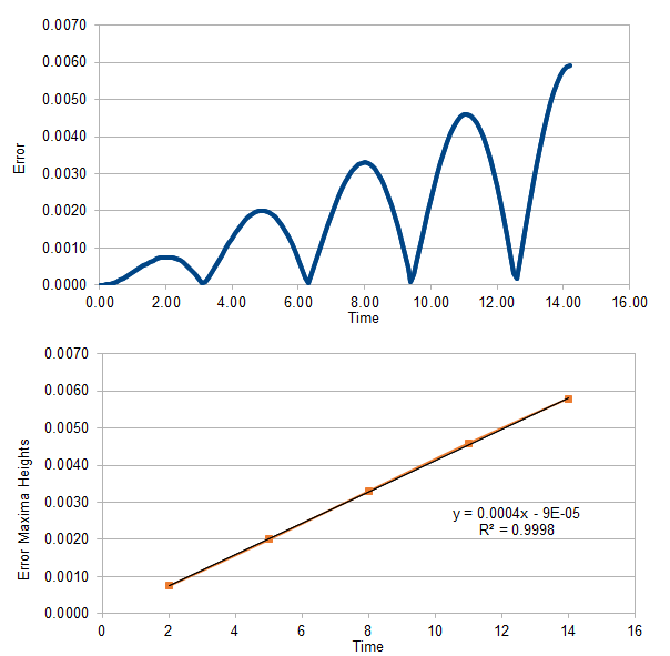
The upper plot shows the error between the analytical and algorithmic values of the displacement. The lower plot shows that a linear line can be fitted through the heights of the error maxima

The equation of the linear fit is shown, and it can be seen that it has a high R² value, indicating that the points correlate with a linear fit very well.

The linear fit was made by estimating the position of the error maxima, and the table of the estimates is given below:

Time (estimate)	Error Height
2	0.000758457
5	0.001999391
8	0.00330076
11	0.00458839
14	0.00578735

Overall, the fit indicates that as time passes, the discrepancy between the algorithmic and analytical methods would increase. However, the gradient for the change is quite small, whereby each increment of time increases the error by roughly 0.0004. Therefore, even if we were to run 1000 iterations of a timestep of 0.1, we would reach a total time of 100, which would give an error of 100 × 0.0004 = 0.04. Compared to the maximum displacement of the oscillator, which is 1.0, this is still only an error of ~ 4%. Therefore, it can be concluded that the error increases at such a slow rate with time that running a sizable amount of timesteps would still allow the simulation to remain within a reasonable approximation to the exact solution. Of course, this applies only to a timestep of 0.1, and the next task explores the effects of changing timestep.

TASK: The displacement for a harmonic oscillator can be described by:

$x (t) = A \cos (ω t + ϕ)$

The total energy of the oscillator can be given by:

$T E = \frac{1}{2} m v^{2} + \frac{1}{2} k x^{2}$

If $A$ , $ω$ and $ϕ$ are all equal to one for the displacement equation, then the analytical total energy is simply half the amplitude squared, which would be 0.5.

Upon choosing different timesteps, the total energy of the algorithm solution oscillated between the analytical total energy and a lower value. It was seen that a timestep equal to or less than 0.2 would not change the total energy by more than 1%. The plot of the total energy of the Velocity-Verlet algorithm solution against time with a timestep of 0.2 is given below:

Oscillating total energy with time of the algorithm solution. The lower bound never reaches more than 1% below the analytical total energy.

It is important to monitor the total energy of a system you are modelling numerically because:

Comparing the numerical total energy values with the analytical values can tell you how accurate your algorithm is at modelling the system.
One needs to observe whether the total energy has converged towards a constant average value, which would indicate that the system has reached thermodynamic equilibrium at its lowest energy state.

TASK: To simulate the interactions between atoms in our simple liquid, the Lennard-Jones potential was used:

$ϕ (r) = 4 ϵ (\frac{σ^{12}}{r^{12}} - \frac{σ^{6}}{r^{6}})$

In order to attain a potential equal to zero, the two terms in the brackets must equal each other.

The separation $r_{0}$ at which the potential energy is zero is:

$r_{0} = σ$

The force at a given separation is attained after differentiating the potential equation wrt $r$ :

$F (r) = 4 ϵ (\frac{12 σ^{12}}{r^{13}} - \frac{6 σ^{6}}{r^{7}})$

The force at $r_{0}$ is:

$F (σ) = 4 ϵ (\frac{12}{σ} - \frac{6}{σ})$

The equilibrium separation $r_{e q}$ is when $F = 0$ . Therefore:

$r_{e q} = 2^{1 / 6} σ$

The potential energy at the equilibrium separation is given by:

$ϕ (r_{e q}) = 4 ϵ (\frac{σ^{12}}{4 σ^{12}} - \frac{σ^{6}}{2 σ^{6}}) = 4 ϵ (\frac{1}{4} - \frac{1}{2}) = - ϵ$

The integral of the potential was evaluated:

$\int ϕ (r) d r = 4 ϵ (\frac{σ^{6}}{5 r^{5}} - \frac{σ^{12}}{11 r^{11}})$

Fixing $ϵ$ and $σ$ to one, the following integrals were evaluated:

$\int_{2 σ}^{\infty} ϕ (r) d r = - 0.0248$

$\int_{2.5 σ}^{\infty} ϕ (r) d r = - 0.00818$

$\int_{3 σ}^{\infty} ϕ (r) d r = - 0.00329$

TASK: In 1 mL of water under standard conditions, the density is approximately 1 g mL^-1, and the Mr of water is 18. The number of molecules can then be calculated:

1/18 × 6.022 × 10²³ = 3.35 × 10²² molecules

Similarly the volume occupied by just 10000 water molecules can be calculated as:

10000 / ( 6.022 × 10²³ ) × 18 = 3.00 × 10^-19 mL

TASK: Since the volume simulated by just 10000 molecules is extremely small, periodic boundary conditions are imposed in order to better approximate bulk liquids. In such a system, an atom at position (0.5, 0.5, 0.5) in a cubic simulation box running from (0, 0, 0) to (1, 1, 1) which moves along a vector (0.7, 0.6, 0.2) would reach the position (0.2, 0.1, 0.7) after applying the periodic boundary conditions.

TASK: Reduced units will also be used for the thermodynamic variables in the simulation.

Using the Lennard-Jones parameters for argon, if the LJ cutoff occurs at r* = 3.2, it is r = 1.088 nm in real units (σ_Ar = 0.34 nm).

The well-depth is $- ϵ$ as calculated before, and its value in kJ mol^-1 can be calculated as:

ⲉ / k_B = 120 K

ⲉ = 1.656 × 10^-21 J

ⲉ = 0.997 kJ mol^-1

The reduced temperature T* = 1.5 in real units would be:

T = 1.5 × ⲉ / k_B= 180 K

Equilibration

In order to start our algorithm we need to assign the initial positions of our atoms. However, liquids don't have long range order.

TASK: Though assigning random positions to the atoms inside the simulation box would achieve the lower degree of long range order characteristic of liquids, this could cause problems. If you have two atoms generated very close to each other for example, the LJ potential will approach infinity at the small separation, generating a large repulsive force between them. If the simulation randomly generates many atom pairs too close to each other, most of the atoms in the system will fly apart from each other at very high speeds due to experiencing strong repulsive forces (i.e. the entire system will fly apart). This is not characteristic of a flowing liquid whereby the atoms are at a separation whereby they are still held together by attractive forces. Or rather, liquids don't spontaneously fly apart, but instead flow.

Therefore, the simulation will start from a simple cubic lattice. If simulated for a long enough time under the correct potentials, the atoms will rearrange into positions more reminiscent of a liquid (i.e. we have melted the crystal)

TASK: Within the input file, the following command creates a simple cubic lattice (one lattice point per unit cell), with a number density of 0.8.

lattice sc 0.8

The output file indicates that the distance between the LPs is 1.07722 (reduced units).

Lattice spacing in x,y,z = 1.07722 1.07722 1.07722

Within a cubic lattice, the LPs all occupy the corners of a cube, but the cube itself contains just one LP (due to sharing the LP with other cubes). Therefore the number density can be calculated as:

1 / 1.07722³ = 0.8

This indeed corresponds to the above input.

A face-centered cubic lattice has 4 LPs for every cube, since the corner LPs are still present (and contribute 1/8 of an LP) and the facial LPs each contribute 1/2 of an LP. For a face-centered cubic lattice with a number density of 1.2, the side length will be (in reduced units):

(4 / 1.2)^1/3 = 1.49380

TASK: For a face-centered cubic lattice, we assume that the following commands were inputted:

region box block 0 10 0 10 0 10
create_box 1 box

create_atoms 1 box

There would be 1000 unit cells contained within the entire box. Since a face-centered cubic lattice has 4 LPs per unit cell, there would be 4000 atoms of type 1 within this simulation box.

TASK: Within the LAMMPS script, the properties of the atoms and the interactions have to be specified through the following parameters:

mass 1 1.0
pair_style lj/cut 3.0
pair_coeff * * 1.0 1.0

The first line sets the masses of the atoms belonging to Type 1 to 1.0 (reduced units). Since a pure liquid is being simulated, only one atom type is present (Type 1).
The second line adds pairwise LJ potential interactions between the atoms, whereby the interaction is calculated only if the atoms have a distance between them which is lower than or equal to 3.0 (reduced units). This cutoff or truncation of the potential is justified, since the integral of the LJ potential between a separation distance of 3.0 and positive infinity was previously calculated to be a small number. This signifies that interactions between atoms at a distance of 3.0 or higher are very small, and that they can be ignored within the simulation.
The third line sets the two coefficients of the LJ potential ( $σ$ and $ϵ$ ) for a pair of atoms. The two asterisks indicate that the coefficients will be applied to the LJ potential of all the pair interactions between the atoms (the equivalent of writing $\sum_{i}^{N} \sum_{i \neq j}^{N}$ ). The coefficients are set to 1.0 in this case.

TASK: Since $x_{i} (0)$ and $v_{i} (0)$ are being specified for this simulation, the Velocity-Verlet algorithm will be used.

TASK: The following lines were typed into the input script

### SPECIFY TIMESTEP ###
variable timestep equal 0.001
variable n_steps equal floor(100/${timestep})
variable n_steps equal floor(100/0.001)
timestep ${timestep}
timestep 0.001

### RUN SIMULATION ###
 run ${n_steps}
 run 100000

The second line creates a variable named 'timestep' and assigns it a value of 0.001. This way, any subsequent line can easily call the variable's value again by typing ${timestep}. This allows for the timestep value to be more easily manipulated and stored in memory so that it can be easily accessed throughout the script. Furthermore, if the value needs to be changed, only the first line which created the variable needs to have the value changed and all subsequent variable calls will change value as well. This is a lot more effective than simply assigning the same value repeatedly to each function call.

The purpose of the subsequent lines is to define more variables, such as the number of steps, to be used later as well. Since defining these variables relies on the values of previous variables, if the value of the previous variables were to change, then these variables would also scale appropriately with the change, which is another advantage of using variables.

TASK: After running the simulation, plots of the energy, temperature and pressure of the simulated liquid system against time were made for when a timestep of 0.001 was used. Additionally, a plot of the energy of the system against time for different timestep sizes was also made:

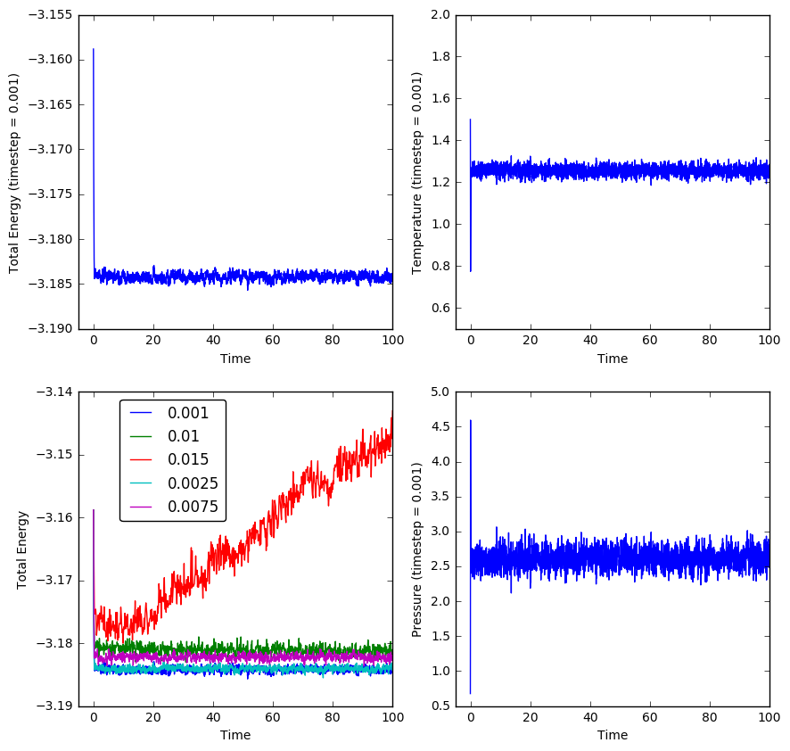
Plots of various thermodynamic variables with time. A plot of the energy of the system against time for various timestep sizes is included at the bottom left.

The system simulated at a timestep of 0.001 can be seen to reach an equilibrium in energy, temperature and pressure very quickly (less than 5.0 time units into a simulation that simulates 100 time units) as all three values rapidly reach an oscillation around an average value.

Using the bottom left plot, it can be seen that the timestep of 0.0025 is the largest timestep that gives acceptable results, since it is larger than the 0.001 timestep but is seen to oscillate approximately around the same average total energy as that of the 0.001 timestep system. The larger timesteps may still give a stable average total energy (excluding 0.015), but these are higher than the average energy indicated by the timestep of 0.0025, which indicates that the higher timesteps have simulated a system which hasn't converged to the lowest energy state, which is the equilibrium state we desire.

Particularly, choosing the largest timestep of 0.015 is a particularly bad choice because it doesn't even give a stable average total energy within the time given. Instead, it gives a total energy that increases further with time, which definitely indicates that the simulated system is not at an equilibrium.

Running simulations under specific conditions (the NpT ensemble)

TASK (Choosing 10 phase points in the NpT ensemble): From the previous simulation under the NVE ensemble, it was seen that a timestep of 0.0025 was the largest that still gave a convergent energy for the system. The average temperature and pressure of the system under the NVE ensemble at a timestep of 0.001 was also calculated after cutting off the first 100 data points (there were 4000 data points for the temperature and pressure, so excluding the first 100 would remove the transient behavior while still leaving enough data points to calculate a reliable average). The following are the averages:

T* = 1.256

P* = 2.615

From these averages indicated by the NVE ensemble, it can be seen that varying the pressure around the value of 2.6 would give reasonable results within the NpT ensemble. Ten simulations of the NpT ensemble were created, whereby a temperature range of 1.6, 1.8, 2.0, 2.2 and 2.4 was chosen and measured at the pressures of 2.5 and 3.0.

TASK: The temperature of the simulated system can be calculated using the equipartition theorem. However, the simulated temperature may differ from that of the target temperature, and so a factor of $γ$ must be multiplied with the velocities for the sum of the kinetic energy of the atoms in order to equalize with the target temperature $𝔗$ . Through this relation, one can solve for $γ$ through the following:

$E_{K} = \frac{3}{2} N k_{B} T = \frac{1}{2} \sum_{i} m_{i} v_{i}^{2}$

$\frac{1}{2} \sum_{i} m_{i} (γ v_{i})^{2} = \frac{3}{2} N k_{B} 𝔗$

$\frac{γ^{2}}{2} \sum_{i} m_{i} v_{i}^{2} = \frac{3}{2} N k_{B} 𝔗$

$γ^{2} = \frac{\frac{3}{2} N k_{B} 𝔗}{\frac{3}{2} N k_{B} T}$

$γ = \sqrt{\frac{𝔗}{T}}$

TASK: The following commands were given to adjust how many times the state of the system was measured.

### MEASURE SYSTEM STATE ###
thermo_style custom step etotal temp press density
variable dens equal density
variable dens2 equal density*density
variable temp equal temp
variable temp2 equal temp*temp
variable press equal press
variable press2 equal press*press
fix aves all ave/time 100 1000 100000 v_dens v_temp v_press v_dens2 v_temp2 v_press2
run 100000

On the second last line, the values 100, 1000 and 100000 signify the way in which the average of a certain variable is calculated. Specifically, there will be 1000 values of the temperature and other variables used to calculate the average value on timestep 100000. Since the simulation only runs for 100000 timesteps, there will only be one average calculated (if the value of 100000 was changed to 10000 for example, there would be ten average values calculated at every 10000th timestep). The value of 100 indicates that the 1000 values used to calculate the average will be taken from every 100 timesteps before the 100000th timestep.

In other words, for our simulation there will be 1000 values chosen from 1000 timesteps, and the first four timesteps of the 1000 timesteps are 100000, 99900, 99800, and 99700. This decrease by 100 timesteps will continue until we have the values from 1000 timesteps. The values sampled will then be used to calculate the average at the 100000th timestep.

TASK: The densities of the various simulations were plotted against the corresponding temperatures and pressures with errors. Additionally, plots of the ideal gas density against temperature were also made for comparison.

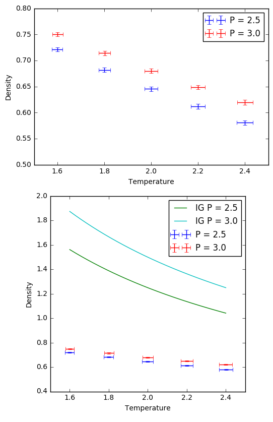
Plots of the density against temperature for the NpT simulations at two different pressures. The lower graph also includes the equivalent plot using the ideal gas equation for comparison.

The simulated densities are much lower than the equivalent densities plotted by the ideal gas law. This is because the ideal gas doesn't take into account any interactive forces between atoms, so atoms could cluster together as close as they want without any interaction occurring, allowing for more dense systems. Our simulation uses the LJ potential to supplie interactive forces between atoms, and it is the large repulsive term in the LJ potential equation that dominates the behavior of the LJ liquid. Since the potential and subsequent repulsive force would increase rapidly with decreasing separation, the atoms in our simulation will always keep a larger distance apart from each other within a certain volume, which would give them a lower density than the ideal gas at the same pressure and temperature.

This discrepancy appears to increase at higher pressures, since the height separation between the simulation plot and ideal gas plot at a pressure of 3.0 is higher than that at 2.5. This is because higher pressures for the ideal gas would continue to compress the atoms closer together without any hindrance from repulsive forces, while our LJ liquid does not change as much in density due to pressure since the repulsive forces are still holding the atoms at a certain distance apart.

Heat Capacity

TASK: The simulation was run using the NVT ensemble so as to calculate the heat capacity of the system. The plot below shows the simulation being run through a range of temperatures and two densities, with the heat capacity per unit volume calculated.

The input file used to calculate the heat capacity is given here: File:Cv origin.in

The heat capacity decreases with temperature as expected. As the temperature increases, more atoms begin to occupy the higher energy states, until almost all of the states are occupied. The energy gained from an increase in temperature would usually go towards increasing the energy level of an atom and not towards the kinetic energy, hence giving the atoms of our liquid a 'capacity to take in heat' without changing temperature. If all the energy states are equally occupied, then the heat capacity will approach zero since there are no more higher energy states left for the atoms to occupy, and so the energy from an increase in temperature will go fully towards increasing the kinetic energy of the atoms.

This is similar to the heat capacity predicted for a two-level system within the NVT ensemble, whereby the plot above is similar to the decay of the heat capacity of the two-level system after it passes the Schottky defect peak. Similar to these plots, the decay of the heat capacity of the two-level system is also due to the fact that both energy levels begin to get equally occupied at higher temperatures.

The increase in heat capacity with increasing density is due to the fact that there are more atoms per unit volume if the density is higher. Therefore, more energy needs to be supplied in order to increase the temperature of a unit volume by one temperature unit, compared to the same volume containing less atoms.

The Radial Distribution Function

TASK: The RDFs for a simulated LJ liquid, solid and gas were calculated and plotted as below:

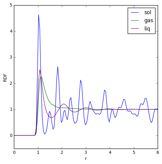
The RDF for the solid has three distinct peaks at the beginning which can be used to find out about the coordination around an atom within the solid. The further peaks all fluctuate around an RDF value of 1, and their fluctuation signifies how the atoms in a solid are held more tightly in place and have long range order such that there is no smooth averaging of their positions.

The RDF for a liquid features three peaks which correspond to the first, second and third hydration shells around an atom. The RDF does not approach zero between these peaks though, indicating that there is a chance of finding atoms between the hydration shells. After the peaks, the RDF averages out to a value of 1, since liquids have no long range order and thus on average the density of a shell a certain distance r from the center doesn't change.

For the gas RDF, there is one peak after which it is subjected to the same averaging effect as the liquid RDF, since gases also lack long range order. The peak is probably due to the gas being surrounded by a sphere of other atoms held together by weak LJ attractive forces, and since there is only one peak rather than the three for a liquid RDF, this signifies that atoms in a gas have less of an attractive force on their neighbors than atoms in a liquid.

The first three peaks of the solid RDF can be used to determine the coordination of the nearest neighbors and second nearest neighbours. The integral of the radial distribution function allows us to physically count how many atoms are included within a volume defined by a certain radius r from the central atom, and it can be overlayed with the normal RDF to give a sense of the coordination number for each of the three peaks.

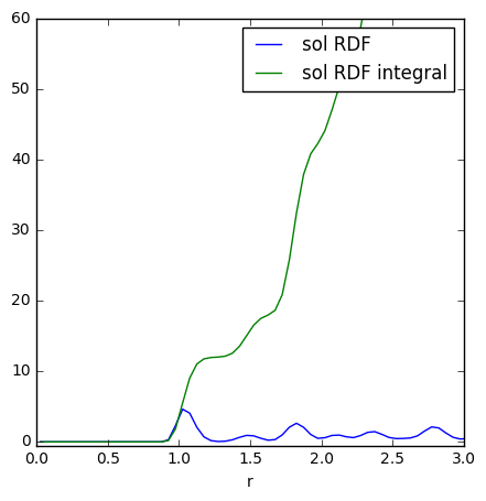
Plot of the solid RDF overlaid with the solid RDF integral

The first peak in the RDF corresponds approximately to the integral value of 12 in the graph, indicating that the first peak of the solid RDF corresponds to a coordination with 12 atoms. The second, smaller peak in the RDF corresponds to the integral value of 18, and if the first 12 atoms are subtracted, this leaves 6 atoms coordinated to the atom from the second RDF peak.

Before deducing the coordination number of the third peak, a diagram can be drawn of the FCC lattice to show which lattice sites the three peaks could correspond to:

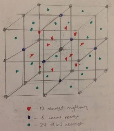
Diagram of an FCC lattice showcasing the coordination of the nearest neighbours

The first RDF peak corresponds do the red dots which form the 12 nearest neighbors to the central atom. The second peak corresponds to the blue dots which form the 6 second nearest neighbours. Finally, the third peak corresponds to the green dots forming the next 24 nearest neighbors. Therefore, the coordination number of the third peak should be 24, and this would correspond to a value of 42 for the integral plot, which can just barely be seen above the third peak since the line is sloping rather than forming a plateau.

The lattice spacing is denoted by the distance to the second nearest neighbors as indicated by the diagram. Therefore, the lattice spacing is r ~ 1.5 since this is the r value for the second RDF peak corresponding to the second nearest neighbors.

Diffusion Coefficient

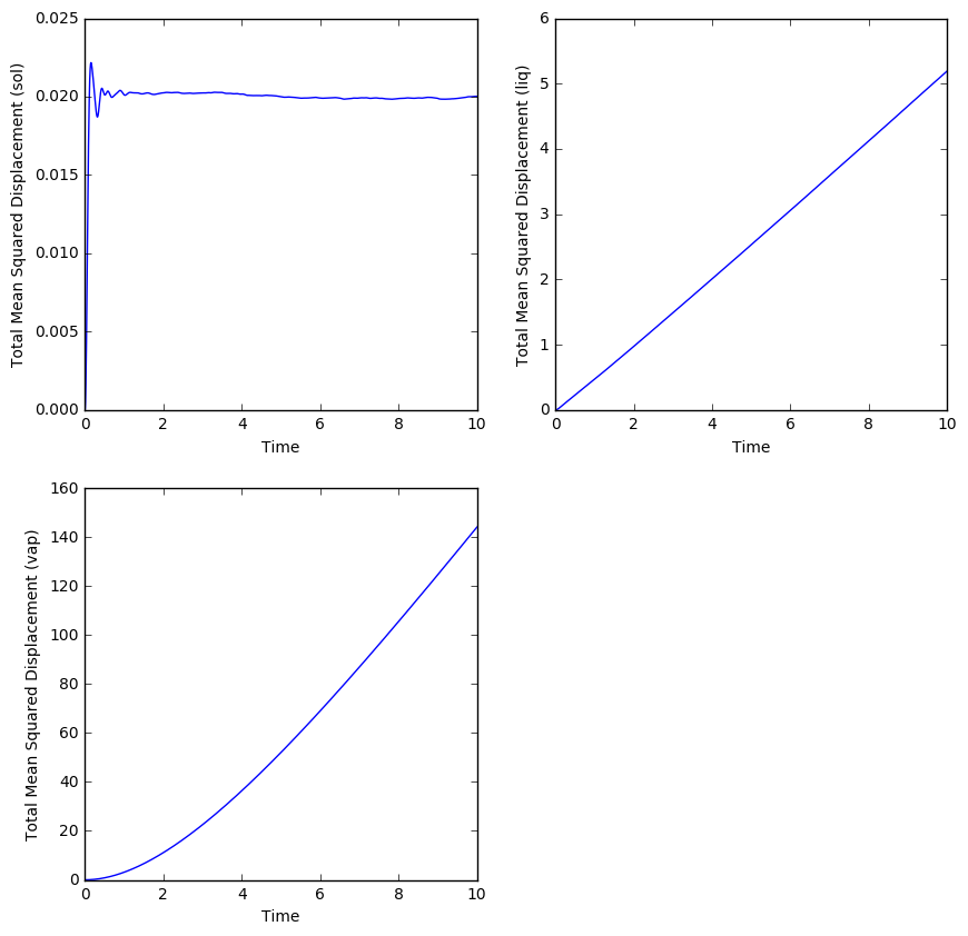
TASK: In order to get a measure of how much our atoms move around in our simulation, we could calculate the diffusion coefficient. The diffusion coefficient can be calculated using the mean squared displacement, and this was calculated for simulations of an LJ solid, liquid and gas. The MSD was then plotted against time:

Plot of the MSD with time for the three states

The diffusion coefficient is directly proportional to the gradient of the MSD with time. With this knowledge, we can make estimates for the diffusion coefficient D.

For a solid, the mean squared displacement is very low (0.02) and stays this way even after a certain amount of time. This is to be expected since atoms in a solid don't displace far from their original position and can only vibrate in place. Since the MSD doesn't really change with time, it has an almost zero gradient, which indicates a diffusion coefficient close to zero, which is also expected because solid atoms rarely (through defects) diffuse throughout a lattice.
For a liquid, the MSD rises with time, since liquid atoms can flow around each other. Therefore, they can eventually reach a displacement quite far from their original positions. The gradient of the plot is estimated to be 0.5, which leads to the following calculation for the diffusion coefficient: $D_{l i q} = \frac{1}{6} (0.5) = 0.0833$
The MSD of an atom in a gas rises more quickly than that of an atom in a liquid, since atoms are free to move around in space within a gas (apart from colliding with other atoms). Therefore, they can very quickly stray far from their original position. If we estimate the gradient from the linear portion of the graph, then: $D_{g a s} = \frac{1}{6} \frac{140 - 120}{9.77 - 8.77} = 3.33$

The diffusion coefficient was also estimated for simulations of the three phases involving one million atoms.

Plot of the MSD with time for the three states using a simulation of one million atoms for each phase

The diffusion coefficient of the solid is once again approximately zero since the gradient of the MSD against time is roughly zero in the plot.
The diffusion coefficient for the liquid has increased slightly, whereby we can calculate: $D_{l i q} = \frac{1}{6} (5.05 / 10) = 0.0842$ .
The diffusion coefficient for the gas is approximately the same as the value calculated for the simulation with less atoms.

TASK: Using the equation for the displacement of a simple harmonic oscillator, we can evaluate the velocity autocorrelation function as follows:

$C (τ) = \frac{\int_{- \infty}^{\infty} A^{2} ω^{2} \sin (ω t + ϕ) \sin (ω (t + τ) + ϕ) d t}{\int_{- \infty}^{\infty} A^{2} ω^{2} \sin^{2} (ω t + ϕ) d t}$

Using trigonometric identities:

$C (τ) = \frac{\int_{- \infty}^{\infty} \frac{1}{2} (\cos (ω τ) - \cos (2 ω t + 2 ϕ + ω τ)) d t}{\int_{- \infty}^{\infty} \frac{1}{2} (1 - \cos (2 ω t + 2 ϕ)) d t}$

We evaluate the integral:

$C (τ) = \frac{\cos (ω τ) t |_{- \infty}^{\infty} - (\frac{1}{2 ω} \sin (2 ω t + 2 ϕ + ω τ)) |_{- \infty}^{\infty}}{t |_{- \infty}^{\infty} - (\frac{1}{2 ω} \sin (2 ω t + 2 ϕ)) |_{- \infty}^{\infty}}$

The integrals involving the sin functions are always bounded to be between -1 and 1, so the much larger $t |_{- \infty}^{\infty}$ term will dominate the fraction:

$C (τ) = \frac{\cos (ω τ) t |_{- \infty}^{\infty}}{t |_{- \infty}^{\infty}}$

$C (τ) = \cos (ω τ)$

The velocity autocorrelation function for the SHO, LJ liquid and solid can be compared as below:

Plot of various VACFs plotted against timestep

The VACF is a measure of how much the current velocity of an atom affects its future velocity (how much they correlate). The minima in the solid and liquid VACFs denote oscillatory behavior for the atoms, whereby the solid phase atoms oscillate in place and reverse their velocities at the end of each oscillation. That is why there are still minima and maxima present for the solid VACF at later times, because the velocity of the atom does have an effect on its future velocity due to influencing its vibration in place. For the liquid phase, the atoms are allowed to flow around each other and diffuse throughout the system, so the correlation rapidly decays exponentially with time since the initial velocity has no effect on the later velocities. There is only one minimum corresponding to one occurrence of velocity reversal for a liquid phase atom, which may correspond to a single collision with another atom before diffusing in the opposite direction. Since liquid atoms don't vibrate in place, there wouldn't be any further minima in the VACF.

The harmonic oscillator seems to have the highest correlation in velocity with time, and its VACF is very different to that of an LJ liquid and solid because the SHO uses a symmetric harmonic potential rather than the anharmonic LJ potential. The oscillator can't diffuse anywhere since it is trapped in the potential well, and its velocities are more correlated than those of an LJ solid because the potential well is symmetric and not subject to more than one kind of interaction, such as the repulsion and attraction simulated by the LJ potential.

Therefore, the vibrations of the SHO are more ordered and restricted to a single dimension than the vibrations of the LJ solid atoms, and the VACF for the SHO is strictly periodic with symmetric minima that, unlike the minima of the LJ solid, never dampen.

The LJ solid could actually be considered a dampened oscillator, since all its atoms are vibrating in place, but since the LJ potential is asymmetric, there is more chance for a random pair of atomic interactions to be different from the last, causing future velocities to 'lose their memory' of the initial velocity. Hence the LJ solid VACF is still lower than that of a perfect oscillator (but still higher than the VACF for a liquid).

TASK: The trapezium rule was used to calculate the running integral of the VACF wrt time. The result was then plotted against time for the solid, liquid and gas simulations.

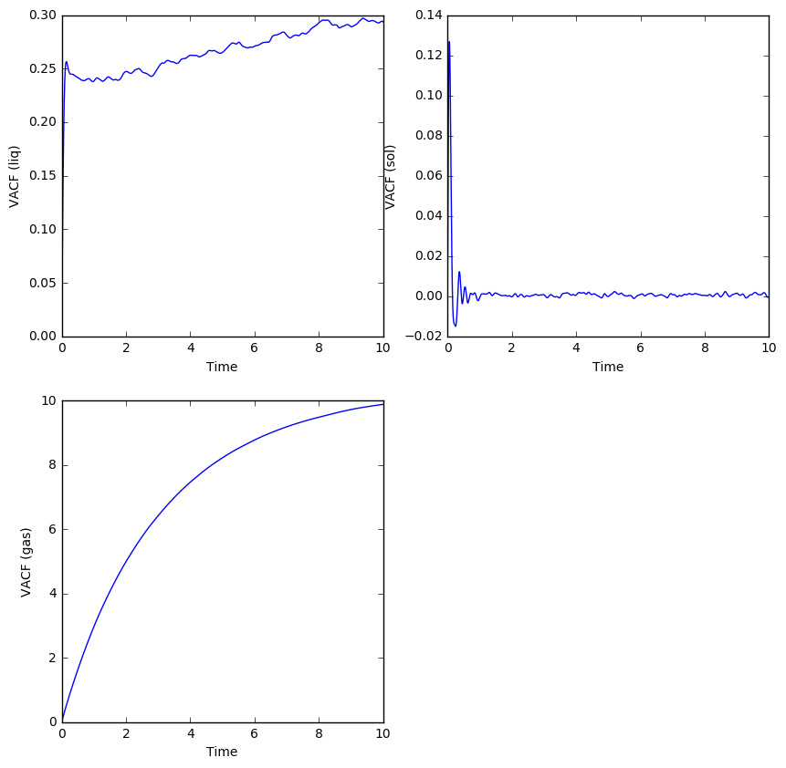
Plot of the running integral of the VACF against time for the three phases

Similar to the MSD, the diffusion coefficients can be estimated from these running integrals. Since the relation of the VACF to the diffusion coefficient is given as:

$D = \frac{1}{3} \int_{0}^{\infty} d τ ⟨ v (0) \cdot v (τ) ⟩$

Then it is evident that the value of the running integral at $t = / i n f t y$ will be equal to the diffusion coefficient multiplied by three. In practice, we simply need to observe when the running integrals in these plots converge to a certain value, and divide the value by three to get the diffusion coefficient.

For the solid, the running integral converges to zero, so the diffusion coefficient must be zero, as expected of atoms which can only vibrate in place.
For the liquid, the running integral converges to a value of about 0.3, which then gives a diffusion coefficient of 0.1 after dividing by three. This is in good agreement with the previously calculated diffusion coefficient of 0.0833 using the MSD.
For the gas, the running integral seems to just converge at a value of about 10, which gives a diffusion coefficient of 3.33. This is almost exactly the same as the value calculated using the MSD, and as expected, the diffusion coefficient of a gas is the highest among the phases, with liquids being in between solids and gas.

Similar to the case of MSD, the diffusion coefficient was also estimated using the running integrals from simulations involving one million atoms.

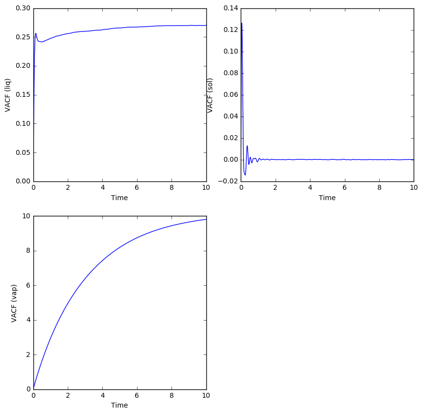
Plot of the running integral of the VACF against time for the three phases using one million atoms for the simulation

For the solid and gaseous simulations, the estimate of the diffusion coefficient will be very similar to that of the simulations that used less atoms.

For the liquid simulation using one million atoms, the noise has at least been smoothed out and we can make out a clearer convergence of the running integral at about 0.27. This gives a value of 0.09 for the diffusion coefficient.

The largest source of error in calculating D from the VACF is possibly from the use of the trapezium rule, which is one of the simplest forms of numerical integration. A more precise method, such as Simpson's rule which uses fitting quadratics, could lead to an estimate of the diffusion coefficient with a smaller error.