Rep:Mod:tw2115transitionstate2017

**Note LOG files are in the appendix** ** Note 2 if gif hasn't loaded or moved click the link**where gifs havent worked the links are in the description**

Introduction

Computer simulations are a useful tool to a chemist allowing a user to set up and then extract data from a system or structure. In this lab Gaussian 09 is used to investigate Pericyclic reactions, most notably the [2+4] Diels-Alder cycloaddition. Gaussian is a sophisticated software, first released in 1970, that enables complex calculations which could not easily be calculated using manual methods.

Aims

The aim of this experiment is to use the gaussian program to investigate a set of Pericyclic reactions. From the simulations I aim to investigate energy barriers, transition states and other factors intrinsic to pericyclic reactions. This investigation also aims to highlight the effects of using different methods to approximate transition states of the reactions and different basis sets. Finally by using computational methods we can compare observations and explain them with molecular orbital theory. In the final parts of exercise 3 I am to use computational methods to make predictions of the most likely products of a reaction with many potential products by computing the reactant and activation energies.

Pericyclic Reactions

In this investigation we look at a variety of pericyclic reactions Diels-Alder, Chelotropic and finally a [2+2] Electrocylcic reaction. Using this set of pericyclics is ideal due to the concerted nature of pericycles reactivity. The single transition state means that once that structure has been found it is possible to go to the reactants or products by creating a small displacement from the transition state on the energy surface. For the Diels-Alder reaction the two reacting fragments are a diene and dienophile. The transition state is formed by HOMO-LUMO interactions of the two fragments. The HOMO of one fragments has the same symmetry as the LUMO of the other fragment allowing interaction to form the transition state. There are 2 of these interactions possible for the HOMO and LUMO of both fragments. There are 2 types of electron demand, normal and inverse. The former is named normal as for a molecule with no heteroatoms we would expect the diene to be more electron rich than the dienophile due to the 2 sets of double bonds. In normal electron demand the HOMO is on the diene. In an inverse demand there is added electron density on the diene this shifts the π bonding orbital to a higher energy and it becomes the HOMO, this is inverse electron demand.

In the first excercise we exam the changes in bond length and structure as the fragments come together and begin to form a 6 membered ring. By comparing the bond lengths with literature values for single and carbon bond lengths we can investigate how the hybridisation of the carbons changes as single bonds turn to double and visa versa. In the first exercise there is also a section on the importance of matching polarity of the molecule when alligning a transition state, another important consideration of the Diels-Alder reaction.

In the second excercise the effects of using a diene with a electron donating hetero atom are investigating and investigating the affect of this on the electron demand of the molecular orbitals. Another feature of the Diels-Alder is that for larger systems there are exo and endo structural isomers possible. The reason for this is when the bong between the diene and dienophile is made two chiral centres are formed with one enantiomer feeling more stabilisation than the other (secondary orbital effects). Using thermochemistry at a B3LYP method we can quantify these results.

The final excercise looks again at the exo vs endo isomers but also considers a chelotropic reaction, by considering the energy of these reactions we are able to make predictions about which products formed and looking at the structures reationalise these predictions.

Finding a transition state

In this investigation two methods were used to predict a transition state that can be optimized through gaussian. The method relies on a guess of the transition state of the required reaction. The concerted nature of pericyclic reactions means that only a single transition state is required this is a useful trait of the pericylic reaction allowing this type of analysis. In the first method used (method 2 in the tutorial) a transition structure is guessed based on chemical knowledge from the system, in this case we know there must be overlap of the frontier molecular orbitals in the diene and the dienophile this tells us that one molecule must be above the other and the p frontier orbitals close to being above each other. Next the bonds are frozen, preventing the fragments drifting apart from not being close enough to the transition structure, and the fragments are optimized in this "guess configuration". The frequencies of the ouput LOG file were checked and a single negative vibrational frequency is indicative of a transition state. Once this arrangement is confirmed as a transition state the true transition state is found by optimising to a Berny transition state with unfrozen bonds and using the keywords opt=noeigen. The output of this calculation is the optimized transition state.

In the other method (method 3) the product structures are drawn and optimised, from this optimization the relevant bonds to get the transition state are broken and hydrogens can be added or removed to ensure the correct valences. From this point method 2 can be employed to get to the final transition state. Method 3 is a useful method for more complicated molecules were the geometry of the transition state is more difficult to guess from 2 molecular fragments. It is employed in the final exercise, exercise 3, due to the increased complexity of using a large diene molecule with a asymmetric transition state.

A note on the energy surface

To run these calculations Gaussian considers potential energy surfaces. When an IRC is plotted the output curve it is a 2 dimensional representation of this surface corresponding to the minimum energy path found by gaussian that navigates the surface from the reactant minimum energy well over an energy barrier to a transition state (characterized by 1 negative frequency, a vibration that lowers energy rather than the usual increase thus a negative force constant, or in terms of the energy surface a point with zero gradient and the second derivative test can be used to check saddle points) . The molecule(s) then pass into a product well which has zero gradient and positive second derivative. To compute this energy surface the program runs calculations over a variety of points quantum mechanically. The level of detail considered by the program, number of approximations and considerations, is determined by the basis set we chose. When we think of the energy surface we often think of a 3 dimensional surface with coordinate q and q'. In reality this energy is a multidimensional surface with co ordinates corresponding to the number of degrees of freedom n. In order to visualise this we combine coordinate axis into a intrinsic reaction coordinate or IRC, this coordinate encompasses a variety of change in geometries corresponding to the different normal modes of the molecule.

Figure 1. A optimisation of a molecule, at first the changes in structure are large but become small near convergance. File:Gifofoptimisingtheproducttw215thomaswebb.gif

Another way of explaining this is by considering a smaller molecule such as water with less degrees of freedom. Water is a bent structure with 3 atoms and thus 3n-6 normal modes where n is the number of atoms, the structure has 3 modes. If we imagine our reaction is the dissociation of the hydrogens from the oxygen this could be envisaged as simply a stretch through the symmetric stretch normal mode to an energy in which the bond dissociates. In reality the reaction may go through a lower path by using motions in different normal modes such as the bonds bending meaning the energy surface is a function of all the possible normal modes. In more complicated molecules this becomes even more difficult to imagine therefore the IRC is a useful coordinate combination of the normal modes that make up the lowest energy path. The gif below is a optimization of a structure, the steps correspond to the molecule travelling through the surface to the minimum via small changes in the geometry and finding the minimum of the normal modes. As the molecule gets closer to the optimum surface the gradient of the curvature is small and therefore the observed changes are small.

Nf710 (talk) 12:46, 1 December 2017 (UTC) This is a nice explanation, but very long and wordy. A diagram would have been very useful here. So gaussian chooses the basis to which it calculates the energy as the normal modes. these are a linear combination of the degrees of freeedom. lots of bends/ streches at the same time. so when you move along the coordinate it looks like a vibration as they are all changing at the same timme.

A note on the transition state

It was previously mentioned that the transition state unique characteristics one of these is the negative frequency. In a normal well all frequencies are positive this is because as the molecule vibrates the energy increases in all directions (normal modes) consider a simple parabola representation. At the transition state there is a vibration towards the products or reactants that will lower the energy of the molecule. If energy is equal to plancks constant times frequency then a negative energy from the vibrations must result in a negative frequency. The gradient at the minima is also zero but the positive curvature in all directions (second derivative equals 0) means that in all directions the change in energy is positive and therefore no negative frequencies should be observed.

Nf710 (talk) 12:46, 1 December 2017 (UTC) And equation woulld have been useful here. this is correct. you could have said a minimum has positive curvature in all dimensions (force constant) and a TS has positive curvature in all except one which is the reaction coordinate. The force constants are obtained by diagonaization of the hessian matrix.

Computational methods

As mentioned previously in the section on the energy surface, in order to construct the surface and perform the optimizations Gaussian must solve quantum mechanics equations (Energy operators). To do this in this experiment 1 of 2 computational methods are used. The frst method was PM6 a semi-empirical method that uses experimental data to fit structures into a better representation.

Nf710 (talk) 12:56, 1 December 2017 (UTC) PM6 is based on HF but used parametrised constants instead of the integrals in the hamiltonian matrix

The other method used is the DFT method. The DFT method is a physics method that stands for density functional theorem. The main difference between DFT and the hartree fock is the hartree fock is calculated from the wavefunction which does not exist in reality, the wavefunction in reality, is a mathematical construct that uses statistical probabilities of where the electron is likely to be to calculate operators such as energy, see above.

The DFT method is chosen to avoid using probabilities of electrons to derive observable such as energy (using a probability as a input will give a probability of an energy or other observable). Instead DFT uses the electron density of a molecule rather than probabilities. The functional part of DFT comes from using functions of the electron density and using this functionality rather than a mathematical wave functions better and for larger molecules a quicker calculation. In this experiment we use B3LYP which is a hybrid of DFT (BLYP). The difference is in the B3LYP there is a 3 term Becke correlation function. This method is commonly considered the best method and a standard in computational chemistry. The basis set used for B3LYP calculations was 6-31(g)d. A 6-31(g) is Pople's basis set and is a very commonly used basis set for gaussian computations. The basis set uses 6 gaussian orbitals for the core orbital, 3 gaussian orbitals for the valence orbital and a further guassian orbital for another valence orbital.

Nf710 (talk) 12:56, 1 December 2017 (UTC) Good attempt, you have definatly read further on this. B3LYP is certainly not the best method in quantum chemistry. It is one of the most versatile. its calculates a DFT hamiltonian and uses a HF calculation to account for the missing exchange correlation term. The best method in quantum chemistry is Coupled cluster theory and it accounts for the electron correlation and hence is the best. but the operation is an infinite taylor expansion so it is hugely expensive.

Another method available is the Hartree Fock method, the hartree fock method makes an approximation of the wavefunction. From this approximation the computer creates a hartree fock matrix calculated from the fock opperator, the matrix is diagonalised. The original matrix is taken the eigenvalues are found and a diagonal matrix is formed (a matrix with eigenvalues only in the positions of the identity matrix (diagonal) by multiplying this by a corresponding matrix of eigenvactors and the inverse of the eigenvector matrix. The vectors are checked for convergence if there is no convergence the matrices are reformed with a different guess of the wavefunction. This method of solving for energy is difficult and only began being used when computational methods were starting to be used..

Nf710 (talk) 13:08, 1 December 2017 (UTC) YUou are talking about the varitational principle and the roothan equations which are key to all of HF based mthods. This would have been much easier to understand if it was in equation form. But you have done well to understand it as I know it is not taught at all in your course.

Exercise 1: [4+2] Diels-Alder Cycloaddition of butadiene and ethene

In this exercise we react a diene (butadiene, typical for these type of reactions) and a dieneaphile (ethene) as a concerted 2+4 cycloaddition figure 2 below.

(Fv611 (talk) Is a butadiene a "typical" reactant for a Diels-Alder? A statement like this needs a reference, but I would also refrain from using vague words like typical in a scientific report. Additionally the log file for the optimised TS is missing so I cannot know whether that optimisation has been done properly.)

Figure 2. Reaction scheme of a simple Diels-Alder reaction of cis-butadiene with ethene, including the transition state structure.

Methodology

Figure 3. Frontier orbitals for the transition state.

For this exercise method 2 as described in the introduction was used. As a typical diels alder a good guess can be made about the transition state. One of the requirements for this concerted pericyclic reaction is that at the transition state the frontier p orbitals are above / below each other figure 3. (Fv611 (talk) Also needs a reference.) From this knowledge of the diels alder transition state a good initial guess of the transition can be made. Once the guess structure was drawn the gaps between the frontier carbons, where bonds were to be formed were positioned around the van der waals radius distance apart (table 3) and the bonds were frozen to prevent the fragments from moving apart and reforming reactants. The structure was optimised to a minimum to optimise the fragments geometries of the suspected transition state. Once optimised the bonds were unfrozen and the molecule was optimised to a berny transition state (Fv611 (talk) Berny is the name of the algorithm used by Gaussian for the optimisation, not a type of Transition State.). To ensure that the transition state was reached the frequencies were changed the vibrations of the fragment were checked. (Fv611 (talk) It is unclear what you mean by "the frequencies were changed".) The transition state should and did have a negative (imaginary) frequency at roughly 950 cm^-1 when this vibration was animated it corresponded to the vibration towards the products which is expected as it is the vibration on the surface that goes down the potential slope towards the products rather than up in energy like the other vibrations.

Once the transition state was identified and checked a intrinsic reaction coordinate or IRC was run which shows a 2D representation of the energy surface between reactants and products. Reactants and products determined by the IRC were optimised to the PM6 level and energy calculations were take, no negative frequencies were observed for the products or reactants. The reactants were also optimised separately for energy calculations at infinite distance between fragments.

MO theory

In this exercise we make use of molecular orbital theory to analyse our reacting fragments and transition state. Using Huckle theory to think of wave functions as sine waves with n-1 nodes the MO's for butadiene and ethene were constructed. Running optimisations on the reactants from the IRC gave the relative energies, and therefore ordering, of these molecular orbitals from this data the fragments of a MO diagram were constructed. For the fragments to interact in the transition state they require having the same symmetry, for a stabilising interaction. This gives 2 possible HOMO-LUMO interactions. The figures below shows these fragments and possible interactions. The MO's in the second figure are the MO's calculated by the guassian software and are based on the orbitals in the first figure.

Figure 4.1. MO diagram for the fragments and transition state of the Diels-Alder reaction. The energies of the fragments and transition state cannot be compared.	Figure 4.2 Same MO diagram as 4.1 with the orbital representations replaced with Gaussian calculated MO's.

(Fv611 (talk) You have calculated the energies correctly, but haven't adjusted the energy levels in the diagram accordingly - why? Also you make no mention of the symmetry of the TS MOs)

Using the checkpoint file from the transition state it is also possible to draw the transition structure MO's. Again the energies of the MO give a method of ordering the MO's relative to other transition state MO's. The interacting HOMO-LUMO form transition state MO's with bonding and antibonding character, the four MO's and their relative energies are given below.

MO no.	16	17	18	19
Visualisation of MO	Figure 5.1	Figure 5.2	Figure 5.3	Figure 5.4
Corresponding MO	Figure 5.1 Lowest energy transition state of the Diels-Alder reaction. Stabilising interaction of 2 Antisymmetric wavefunctions LUMO of ethene and HOMO of diene	Figure 5.2 Stabilising interaction of the two symmetric wavefunctions (HOMO of the transition state). HOMO of the ethene fragment and LUMO of the diene fragment.	Figure 5.3 Destabilising interaction of the symmetric wavefunctions (LUMO of the transition state).	Figure 5.4 Destabilising interaction between the asymetric wavefunctions.
Relative Energy	-0.32756 au	-0.32533 au	0.01732 au	0.03067 au

Table 1. Table containing images of the real MO's calculated by Gaussian and there MO representations. The relative energies compare the energies of each MO relative to each other, again these cannot be compared to anything except other orbitals.

The images above visualise the interaction of the two sets of fragment orbitals with the same symmetry (AS-AS / S-S). Symmetry is important to ensure there is a net constructive overlap between the two combining orbitals. For interactions of the same symmetry there is a constructive overlap and the overlap integral S_AB is nonzero. Equations 1-6 below shos the overlap integral S_AB as a integral of the two wave functions. If the orbitals have mismatched symmetry then the overall integral is asymmetric and therefore integrates to 0. This is because integrating an odd function is equal to 0.

Ψ(AS) x Ψ(AS) = Ψ(S) equation 1

Ψ(S) x Ψ(S) = Ψ(S) equation 2

Ψ(S) x Ψ(AS) = Ψ(S) equation 3

$S_{AB}=\underset{}{\overset{}{\int }}symmetric\ne 0$ equation 4

$S_{AB}=\underset{}{\overset{}{\int }}{\psi }_S{\psi }_{S}d\tau \ne 0$ equation 5

$S_{AB}=\underset{}{\overset{}{\int }}{\psi }_S{\psi }_{AS}d\tau =0$ equation 6

Bond Lengths

Figure 6. Atom labelling of the cyclohexene product.

The table below shows the bond lengths between the carbons

	C1-C2	C2-C3	C3-C4	C4-C5	C5-C6	C6-C1
Reactants	1.33344	1.47083	1.33343	inf	1.32737	inf
Transition state	1.37980	1.41124	1.37965	2.11577	1.38172	2.11394
Products	1.50034	1.33766	1.50034	1.54003	1.54076	1.54003

Table 2. Table of carbon carbon bond lengths in the reactants, transition state and products (Fv611 (talk) The VdW radius of carbon isn't 2.2.)

	Bond length
C-C Single bond	1.544
C=C Double bond	1.33
Van der waals	2.2

Table 3. Table of the reported values of single bonds, double bonds and the van der waals radius of carbon.

As the reaction goes from reactants to products there is stretching and compression of bond lengths. The C1-C2 (end of the diene) is a good example of this change, The bond starts as a sp² hybrid carbon double bond. As the molecule goes to the transition state the bond length extends, when the molecule is at the transition state the bond length is between a single carbon sp³ and double carbon sp² bond. As the molecule goes from the transition state to the reactants the bond extends further to the full single bond length in the product. This situation is mimicked in the C3-C4 (other end of the diene) and the C5-C6 double bond in the ethene. The opposite occurs for the bond between carbon 2 and carbon 3. For these bonds the carbons come closer and the transition state bond length is shorter than the sp³ length. The final bond length is consistent with a carbon carbon double bond. For the bonds that link the fragments, initially as reactants we assume the fragments are infinitely far apart, at the optimised transition state the carbon carbon bond length is close to the van der waals radius, (there is a weak attraction between the atoms). As the molecules go to the products these bonds shorten to single carbon carbon bonds. The motion of the atoms and the changes in the bond lengths is shown in the gif below.

Figure 7. Animation of the Diels-Alder reaction from reactants through the transition state to the products.

The gif also shows the change in the angle, in the reactants the ends of the dienes are sp² hybridised orbitals, the p orbital is a frontier orbital and key to the reaction. As the reactant approaches the transition state the angle between the carbon and the hydrogen changes from 120^o visualising that a change in hybridisation is occurring.

(Fv611 (talk) You forgot to discuss the timings of bond formation)

Matching Polarity

(Fv611 (talk) How do you know that the struggle in reaching a transition state is due to the polarity and not to something else (eg. sterics)? This kind of discussion needs referencing too.)

Figure 8. Diagram showing the polarities of the fragments

In this Diels-Alder reaction the symmetry plane through each molecule means there is no constraint on which end of the fragment reacts where. When substituents are added to either the diene or dienophile a polarity is introduced into the fragment. In this example a amine (Electron donating group) and a chlorine atom (electron withdrawing group) are added asymmetrically. The figure right shows the induced polarity of the fragment orbitals. Fragments with an intrinsic polarity such as those in figure 8 require that these polarities are matched, this is something that must be considered in the first guess of the transition state.

The table below shows matched and mismatched optimisations to a transition state.

Alignment	Mismatched polarity	Matched polarity
	Figure 9.1 Mismatched polarity of the diene and dienophile the molecule doesn't go to a transition state.	Figure 9.2 Matched polarity of the fragment orbitals in this animation a transition state is found. File:Gif of matchtw21152114.gif

Table 4. Animations of the optimisation to a transition state of a diene and dienophile with heteroatoms allowing control of the polarity of the fragments.

The gifs above show that the transition state can only be found when the polarity is matched. For this example the matched polarity places the ammonia and chlorine at opposite ends of the transition state.

Exercise 2: Exo vs Endo Diels-Alder Cycloaddition

In this excercise a more complicated example of the diels alder is modelled. In this system there are two orientations that the dienophile can align itself with diene fragment. The reaction scheme below shows the product of both these alignments and the transition states associated with them.

Figure 10. Reaction scheme of exercise 2 including the transition states.

Methodology (PM6)

In this exercise method 2 was used similar to exercise 1. From a benzene molecule the cyclohexadiene fragment was constructed . Next the 1,3 dioxole was constructed using a cyclopentene fragment and inserting divalent oxygen. Using the same type of guess as used in the first excercise the transition state was approximated and the distances between the frontier atoms set to the van der waals lengths and frozen. This optimisation yielded the optimised structures of the fragments in the guessed transition state, a single negative frequency around -550 cm^-1 for both isomers proved the guess was a transition structure. As previously the bonds were unfrozen and the fragments were optimised to the berny transition state. Again both transition states gave a single negative frequency, from this point 2 calculations were run on both of the transition structures, the B3LYP optimisation is given below. Using the PM6 Berny Ts calculated previously an IRC was run. From the IRC the last (or first depending on the direction taken at the transition state) point was taken as the product. This product was taken and optimised to the PM6 level.

Methodology (B3LYP Energy calculations)

For looking at the energy and thermochemistry of the reaction the B3LYP basis was used to gain a better accuracy at the cost of computational expense. The first set of molecules that were optimised with the B3LYP method was the reactants. By constructing the diene and dineophile seperately both structures could be optimised and the energys added, it is important to run these simulations seperately as there must be no potential interaction between the fragments. Before both fragments ran the symmetry was broken by slightly modifying the dihedrals this prevented negative frequencies (happening upon another transition state between geometries of the reactants due to symmetry). For both these calculations the PM6 method was used to first clean up the structure and speed the B3LYP calculation.

For the transition states the PM6 optimisation to a Berny transition state was taken and the resulting molecule was optimised using a B3LYP method. Running the IRC on the B3LYP would have been far to computationally expensive and many of the intermediate structures between the transition state and products are unnecessary especially to a B3LYP approximation. For this reason the IRC was ran as a PM6 and the final resulting geometry was optimised using a B3LYP calculation thereby avoiding hours of needless calculations. It is also important that the IRC was run using the PM6 Transition state, the reason is because the IRC method must match that used to find the transition state to ensure the surface is the same and the two calculations agree on the transition state having a gradient of 0 on the same surface. The reactants of the IRC were subject to a single point energy calculation this allowed calculation of the molecular orbitals and their energy relative too each other. The MO's and their energy for the transition state can be extracted from the optimisation calculations on the transition state either B3LYP or PM6.

MO Theory

The MO diagram for this reaction is heavily based on that in part 1. The diene in the cyclohexadiene has the same frontier p orbitals as in the butadiene example. Similiary the dioxole pi bond has only 2 different MO's (bonding and antibonding). The molecular orbital diagrams for the exo and endo products are given below.

Figure 11.1 MO Diagram of the Endo Diels-Alder transition state.	Figure 11.2 MO Diagram of the Exo transition state.

(Fv611 (talk) Like in part one, you know the relative energies but haven't adjusted the MOs accordingly. Luckily in this case the inverse electron demand makes the order of your reactants' FMOs correct, but the bonding TS MOs should both be higher in energy than the diene's HOMO and the antibonding TS MOs should both be lower in energy than the dienophile's LUMO.)

Table 5. MO diagrams of the endo and the exo fragments and transition states.

In the table below are images of the transition state MO's along with a MO representation of the orbitals.

MO	40 (ENDO)	41 (ENDO)	42 (ENDO)	43 (ENDO)
	Figure 12.1	Figure 12.2	Figure 12.3	Figure 12.4
	Figure 12.1	Figure 12.2 Oxygen p orbitals are in red.	Figure 12.3	Figure 12.4 Oxygen p orbitals are in red.
MO	29 (EXO)	30 (EXO)	31 (EXO)	32 (EXO)
	Figure 13.1	Figure 13.2	Figure 13.3	Figure 13.4
	Figure 13.1	Figure 13.2	Figure 13.3	FIgure 13.4

Table 6 MO representations of the transition state combinations of HOMO and LUMO fragments orbitals, above them are images of the MO's calculated by Guassian.

MO theory allows us to describe this reaction as a inverse demand Diels-Alder cycloaddition. The dienophile, dioxale fragment, is electron rich due to an increased electron density via the oxygen hetero atom. As a result of this increase in electron density on dienophile, the moleculer orbital energy is increased. This increase means that the pi bonding orbital is shifted above the HOMO of the diene and thus becomes the HOMO of both fragments. This is known as inverse electron demand.

The HOMO on the dienophile will interact strongly with the LUMO on the diene. In the previous excercise the highest energy occupied molecular orbital for the fragments was on the diene this is normal electron demand, the diene is more electron rich then the alkene fragment.

Nf710 (talk) 13:11, 1 December 2017 (UTC) Thisis correct if you wanted to look at this quantitativelyyou could have done a single point energy on the reactants (on the same potential energy surface)and looks at the ordierng of MOs tehre

Thermochemistry

By using a B3LYP method to optimise structures it was possible to extract thermochemistry information from the guassian outputs. As mentioned previously in the method section the reactants were calculated as seperate gaussian input files the data for the reactants is given below.

Reactants

Molecule	Free Energy (hartrees)	Free Energy (kj mol-1)
1,3 Dioxole	-267.0686	-701,188
Cyclohexadiene	-233.3243	-612,592
Sum of reactants	-500.3929	-1,313,781

Table 7. Thermochemistry data from the reactants.

Endo Product

Molecule	Free Energy (hartrees)	Free Energy (kj mol-1)
Transition state	-500.3321	-1,313,621
Product	-500.4187	-1,313,849
Activation Energy	0.0608	159.63
Reaction Energy	-0.0258	-67.73

Table 8. Thermochemistry data from the endo reaction.

Exo Product

Molecule	Free Energy (hartrees)	Free Energy (kj mol-1)
Transition state	-500.3291	-1,313,614
Product	-500.4173	-1,313,845
Activation Energy	0.0638	167.51
Reaction Energy	-0.0244	-64.062

Table 9. Thermochemistry data from the exo reaction.

The table above shows the energies calculated from the reactants, transition states and products (method(B3LYP)). The table also shows the energy from the reactants to the transition state (activation energy barrier) and the reaction energy (product energy minus the reactant energy). The energy of the products is more negative than the free energy of the reactants so if the activation energy is met this reaction will happen spontaneously. The equation below shows the arhenius equation. We can see in the table above that the activation energy is less in the endo reaction using the Arrhenius equation this corresponds to a faster rate of reaction, this means the endo product is the kinetic product of the reaction.

$K=A{e}^{\frac{-Ea}{RT}}$ equation 7: The Arhenius equation

Comparing the energy of the final exo/endo product energy, the endo product has a lower energy and is therefore more thermodynamically stable. The endo product is the the thermodynamic product of this reaction, the endo product is both the thermodynamic and kinetic product.

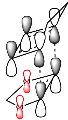
To consider why this is we first look at the molecular orbitals of the transition state table 6. The main difference between the molecular orbitals in the exo and endo transition states is the contribution from the oxygen p orbitals in the endo transition state. Table 6 also shows a representation using molecular orbitals and the images of the actual orbitals predicted. This affect is observed in the orbitals 41 and 43 and represented with red p orbitals. The effect is secondary orbital overlap from the oxygen p orbitals and 2 of the molecular orbitals from the diene fragment. The overall effect of this is a stabilisation of the transition state and a lowering of the orbital energies. This secondary orbital effect is responsible for the more negative (stable) transition state in the endo transition state. The stabilisation corresponds to roughly 8 kj mol^-1 in this system.

To rationalise the thermodynamic stability of the endo product relative to the exo product one must consider the sterics of the final products. Below are representations of both molecules.

ISOMER	EXO product	ENDO product
	Figure 14.1 Exo product (side view).	Figure 14.2 Endo product (side view).
Relative Free energy difference of product (kj mol-1)	+ 4 kj mol-1	0

Figure 15. Guassian calculated MO of the product showing the retention of secondary orbital overlap stabilisation.

Table 10. Comparison of the exo and endo products and their energies.

The energy calculation shows that the difference in the products is only small and most likely comes from the flagpole type steric strain in the exo product between the top hydrogen. Table 10 also shows a molecular orbital from the product. The molecular orbital shows that in the product there is still secondary orbital between the oxygen atoms and the pi orbitals from the C=C bond in the newly formed cyclohexene ring. This interaction is not possible in the exo product and is a further effect that stabilises the endo product relative the exo product.

Italic text

Nf710 (talk) 15:09, 1 December 2017 (UTC) This was a good section. I liked your use of the arrehenius equation and your argument for steric is really good. Your energies are also correct.

Exercise 3: Reaction of o-Xylylene with SO_2, Diels-Alder vs Chelotropic cycloadditions

In this excercise Diels-Alder reactions are performed between a symmetric diene and a inorganic dienophile, sulphure dioxide. This exercise looks at the differences again between the endo and exo reaction pathways but also investigates cheloptropic cycloaddition as an alternative reaction path to the Diels-Alder reactions investigated previously. In the later stages of this exercise an alternative diene in the reactants is investigated.

Figure 16. Reaction scheme for exercise showing the alternate reaction paths and the transition states.

Methodology

In this experiment method 3 was used, this meant the product of the reactant was optimised first to a PM6 level, ensuring to break any symmetry by altering the dihedral. Once optimised with no negative frequencies observed the relative bonds on the ends of the fragments were broken and the relevant hydrogen's added ensuring they are planar (sp² hybridisation). The optimised sulphur dioxide fragment was placed above the planar molecule at the relevant van der waals radii. The atoms that are to form bonds were frozen and the molecule optimised to a minimum at a PM6 level. The bonds of the product were unfrozen and the optimised transition state guess was optimised to the true Berny transition state (1 negative frequency). IRC paths were calculated for the reaction and from these paths the product structure was obtained and further optimised with a PM6 optimisation.

(Watch out that Berny is an optimisation algorithm, not directly related to the TS Tam10 (talk) 16:21, 27 November 2017 (UTC))

Reaction Energies

Reactants

Reactant	Free Energy (Hartrees)	Free Energy (kj mol-1)
5,6-dimethylenecyclohexa-1,3-diene	0.1780	467.3
Sulphur Dioxide	-0.1186	-311.4
Sum of Reactants	0.0594	155.9

Table 11. Thermochemistry of the reactants of both reactions

Endo Diels-Alder

State	Free Energy (Hartrees)	Free Energy (kj mol-1)
Transition state	0.0905	237.6
Product	0.0217	57.0
Activation Energy	0.0311	81.6
Reaction Energy	-0.0377	-99.0

Table 12. Thermochemistry of the Endo Diels-Alder reaction.

Exo Diels-Alder

Energy of	Free Energy (Hartrees)	Free Energy (kj mol-1)
Transition state	0.0920	241.5
Product	0.0214	56.1857
Activation Energy	0.0326	85.6
Reaction Energy	-0.0388	-101.9

Table 13. Thermochemistry of the Exo Diels-Alder reaction.

Chelotropic

Energy of	Free Energy (Hartrees)	Free Energy (kj mol-1)
Transition state	0.0990	259.9
Product	0 (-0.000002)	0 (-0.00521)
Activation Energy	0.0396	103.9698
Reaction Energy	-0.0594	-155.9

Table 14. Thermochemistry of the chelotropic reaction.

The first observation made from the thermodynamic data collected about the systems is out of the three possible reactions the chelotropic forms a considerably more stable product that either of the Diels-Alder reactions. If performing this reaction experimentally the chelotropic product is the thermodynamic product, the large stability gained for this is most likely the symmetry of the product and in the 5 membered ring. In the Diels-Alder the introduction of 2 different heteroatoms into the ring creates distortion. This product is however kinetically unfavourable, when the energy barrier is compared with the diels alder reaction the barrier is almost 20 kj mol^-1 than the kinetically unfavourable exo transition state. The arhenius equation tells us that this big increase in activation energy will exponentially decrease the rate at which the product is formed. It is unlikely much of this product would be formed at standard conditions experimentally the Diels-Alder product would dominate kinetically. This is an example whereby using computational methods it is possible to make predictions about a chemical system in this case we predict that although thermally more stable the Diels-Alder would be a dominate reaction path for the same set of reactants.

(The stability likely comes from lower strain of the 5-membered ring due to the size of the sulfur atom, as well as the retention of both S=O bonds Tam10 (talk) 16:21, 27 November 2017 (UTC))

Comparing Diels-Alder reaction it is observed that the endo reaction is again the kinetic product due to its lowered activation energy barrier. However the product is no longer the most stable product out of the exo and endo pair, the exo product is more stable when comparing the two diels alder reaction paths. There is however a large difference in the activation energy and the exponential nature of the arhenius equation tells us this will have a big effect on the rate of forming products. It would be expected that at lower temperatures (more emphasis on the activation energy term in the arhenius equation) that the endo product would again dominate the reaction. It is likely the endo product would be the major product of this reaction being carried out experimentally (especially at lower temperatures - Kinetic conditions).

(You will likely get a mixture of endo- and exo- as the differences in energy of the products is negligible. Tam10 (talk) 16:21, 27 November 2017 (UTC))

Reaction Energies at the other diene.

Exo

	Free Energy (Hartrees)	Free Energy (kj mol-1)
Transition state	0.1051	275.9
Product	0.0673	176.7
Activation Energy	0.0457	120.0
Reaction Energy	0.0079	20.7

Table 15. Diels-Alder thermochemistry at the less favoured Exo site.

Endo

	Free Energy (Hartrees)	Free Energy (kj mol-1)
Transition state	0.1021	268.1
Product	0.0656	172.2
Activation Energy	0.0427	112.1
Reaction Energy	0.0062	16.3

Table 16. Diels-Alder thermochemistry at the less favoured Endo site.

The table above shows the thermodynamic data for the Diels-Alder reactions at the other diene in the molecule. The most important difference between this data and the previous diels alder is the change of sign in the reaction energy. In the previous set of reactions the cycloaddition corresponded to a lowering of energy in the system. At this site the reaction corresponds to a increase in the energy of the system and endothermic reaction. This is thermodynamically unfavourable at this position, there is also a substantial activation barrier to forming these products making them kinetically unfavourable as well as thermally. From this computational calculation we can predict when these reactants are put together experimentally we do not expect to see any of the diels alder products at this diene.

In this reaction to form the transition state the aromaticity of the molecule must be borken in the first reactions the aromaticity is restored when the products are made by the formation of the double bond in the cyclohexadiene ring, when reacting at this site the aromaticity is lost and this is responsible for the increase in the energy from the reactants to the products.

(o-xylylene is anti-aromatic

Intrinsic Reaction Cooordinate

As mentioned in the introduction the intrinsic reaction coordinate is a 2 dimensional representation of the minimum energy path from reactants to products. In this exercise we start with the transition state (a saddle point on the potential energy surface) the IRC will look and travel down the minimum energy path on either side in steps reporting the geometries. By combining the geometries as frames of a movie it is possible to run them sequentially and form a continous visual representation from reactants through the transition state to product, these representations are given below as fig files.

Exo DA	Endo DA	Chelotropic
Figure 17.1. Exo Diels-Alder animated IRC path.	Figure 17.2. Endo Diels-Alder animation of IRC path.	Figure 18. Chelotropic Diels-Alder animation of the IRC path.

Table 17. comparison of the animated IRC paths (geometries) for Diels-Alder and chelotropic reactions.

The gifs above allow the computational chemist to visualise observe the reaction and details of the reaction. For example the gifs show that for the exo and endo Dials-Alder have asynchronous bond formation due to the lack of symmetry of the fragments. In the chelotropic reaction the bond formation is synchronous this is because the symmetry of the fragments mean there is no reason why one bond should be made before the other. The gif of the exo diels alder reaction is in the reverse direction this is because at the transition state of the molecule there is a 50:50 chance of the minimum the tested being products or reactants, the direction makes no difference and can easily be reversed. The figure below shows plots of the reaction coordinate against the free energy. In this figure the energies used are from optimised structures at the PM6 level. The intrinsic reaction coordinate plot forms a curve due to the number of points taken. In the plot below only the reactants, transition states and products are shown, these energies are the most important for comparing reaction energies. The figure allows comparison of the stability of products as well as a visual comparison of the activation energies.

Figure 19. Visualisation of the reactant and activation energies. All energies are relative to the product energies.

(Your energies here are in Hartrees, not kJ/mol)

The energies in the figure above are relative to the reactant energy which has been set to 0 for the purposes of this diagram.

Further work [2+2] 4π Electrocyclic pericyclic reaction

In this section a [2+2] electrocyclic reaction is run. With reactions of this type we can investigate the effects of con and dis rotary mechanisms.

Figure 20. Reaction scheme for the [2+2] electrocyclic pericyclic reaction.

Methodology

Figure 21. Geometry of the found transition state.

This calculation was far more difficult to find the transition state. For this to work method 3 was used (due to the large rings on the transition state). The product structure was first drawn (I didn't want to show preference on a conformer for the cyclohexane rings therefore symmetry broken benzene was chosen and the rings could shift into their own optimum geometries) the structure was optimised with a PM6 optimisation + frequency.The frequencies were checked and all were positive.

(This is a risky strategy. Gaussian might land in a local minimum, not the true global minimum. For the purpose of demonstration, what you have done is fine but ideally you should test all conformers if possible Tam10 (talk) 16:33, 27 November 2017 (UTC))

Next the carbon carbon bond that is formed in the reaction was broken and the distance was set to 2.0 angstrom (any distance greater pushed the rings apart and was not close enough to induce the transition state, the actual transition state had a bond length of 2.3 angstrom). This was minimised to a minimum with the bonds frozen. This gave a single negative frequency. The structure was then unfrozen and optimised to the Berny transition state. For the first few runs this yielded 2 negative frequencies. The symmetry of the minimised molecule was slightly altered via the dihedral and the structure was reoptimised to transition state yielding only 1 negative frequency corresponding the correct stretches. It was also important to ensure the hydrogens on the frontier carbons were on the same face. IRC of this reaction was run, this was a length procedure due to the amount of optimisations required to get to the energy minima. To observe how the orbitals move and twist from reactants to products, points were chosen along this path and single point energy calculations were run to visualise how the orbitals change and categorise the reaction as con vs syn (as well as the gif below of the reaction). At first I was surprised that the two cyclohexane rings should share the same face however this is a necessary requirement due to the hydrogens needing to be on the same face (the cyclohexane are conrotation).

(It would be nice to see how these orbitals change as the reaction progresses Tam10 (talk) 16:33, 27 November 2017 (UTC))

Figure 22. Animation of the IRC path (minimum energy path) from the products to the reactants from the transition state.

Woodward Hoffman Analysis

The figure above is an animation of the geometries the molecule passes through on the IRC from the product going back to the reactants (wouldn't upload in the other direction). What is clear from the animation is that the hydrogens on the carbons move together in the same direction, left in the animation from products to reactants and thinking in reverse would twist right together going to products. This observation is rationalised by Woodward Hoffman analysis. For a reaction to be accessible by thermochemistry there must be either (4q+2) suprafacial electrons or (4r) anterfacial. For this reaction the product, figure 20, has 4 pi electrons and therefore to be thermally allowed must be have anterfacial connectivity this is shown in the figure below.

Figure 23. Diagram showing how the frontier p orbitals connect and come together in the electrocylic reaction.

(You should use the correct phases for this diagram to explain why the reaction proceeds with conrotation Tam10 (talk) 16:33, 27 November 2017 (UTC))

In this example the reaction is calculated as a thermal reaction calculated from the ground state. If the reaction was excited using photo chemistry the disrotatory product would be formed according the woodward hoffman rules. The connectivity in the figure above is anterfacial this is because the p orbital lobes on opposite faces are connected.

(+10% Tam10 (talk) 16:33, 27 November 2017 (UTC))

Conclusions

In this investigation the importance of computational methods have been shown. This best shown by exercise 3 were for a reaction with multiple potential products we use gaussian to calculated the energies of the reactions and we can therefore make conclusions about what sort of products we can hope to obtain from running this experiment experimentally. This makes gaussian an extremely useful tool for the experimental chemist to make predictions. Guassian also has the feature of drawing MO diagrams, this means for a reaction such as 2 where one reaction is favoured over the other, by looking at the molecule orbital data calculated by gaussian the chemist can look for effects such as secondary orbital overlap that can explain experimental observations. This excercise shows the importance of Gaussian for not only the theoretical chemist but also the experimental chemist looking for data on a reaction. By optimising molecules gaussian also offers a visualisation of the molecule this is useful as guassian considers the van der waals radii on each atom and thereby steric energy increases are considered by looking at the visualization it is possible to look for steric effects.

Appendix

Exercise 1.

Computation	LOG File
1,3 butadiene optimisation PM6	File:Tw2115 Butadiene Optimisation PM6.LOG
Optimise guess transition to minimum (FB) (PM6)	File:TW2115 First optimisation of TS to minimum.LOG
Optimise transition state to TS Berny (PM6)	TW2115_optimise_to_Berny_TS.LOG ‎
IRC of reaction	File:TW2115 IRC Ex1.LOG
IRC reactants optimisation (PM6)	TW2115_Reactants_of_IRC_opt.LOG
IRC products optimisation (PM6)	TW2115_IRC_product_opt.LOG

Polarity extension

Computation	LOG File
Optimisation of Ts to minimum (mix match)(FB)(PM6)	File:Tw21151ST OPTIMISE TO MINIMUMmismatched.LOG
Optimisation of TS to minimum (matched) (FB)(PM6)	File:TW2115optimisetheCORRECT LINE UP.LOG
Optimisation of TS to Ts Berny (matched) (PM6)	File:Tw2115extensionOPTIMISE TRANSITION STATE.LOG
IRC of matched	File:Tw2115IRC OF EXTENSION.LOG

Exercise 2.

Exo

Computation	LOG File
Optimisation of TS guess to minimum (FB) (PM6)	File:TW2115 Ex2 Exo opt to min.LOG
Optimisation of TS minimum to TS Berny (PM6)	File:TW2115 optimisation to TS Berny.LOG
Optimisation of TS Berny PM6 to Ts Berny (B3LYP)	File:Tw2115 Ex2 Exo TS B3LYP.LOG
IRC of PM6 Transition state	File:Tw2115 IRC Ex2 EXO.LOG
IRC reactant single point energy (PM6)	File:TW2115 Ex2 Exo reactants SPE.LOG
IRC products optimised Exo (PM6)	File:Tw2115 Ex2 EXo IRC product optimised PM6.LOG
IRC products optimised Exo (B3LYP)	File:Tw2115 Exo Ex2 IRC product B3LYP.LOG

Endo

Computation	LOG File
Optimisation of TS guess of Endo to minimum (FB) (PM6)	File:Tw2115 Ex 2 Endo first opt to min.LOG
Optimisation of TS minimum to TS Berny (PM6)	File:TW2115 Opt Endo to Ts Berny PM6.LOG
Optimisation of TS Berny PM6 to Ts Berny (B3LYP)	File:Tw2115 opt transition to B3LYP.LOG
IRC of PM6 Transition state	File:TW2115 IRC of endo ex 2.LOG
IRC reactant single point energy (PM6)	File:TW2115 IRC Reactants Endo SPE.LOG
IRC products optimised Endo (PM6)	File:TW2115 ENDO PRODUCT OF IRC PM6.LOG
IRC products optimised Endo (B3LYP)	File:Tw2115 endo product of IRC at B3LYP.LOG

Reactants

Computation	LOG Files
Optimisation of Dioxole reactant (B3LYP)	File:Tw2115 dioxole optimised to BLY.LOG
Optimisation of cyclohexadiene (PM6)	File:TW2115 opt of HEXADIENE PM6.LOG
Optimisation of cyclohexadiene (B3LYP)	File:TW2115 OPT HEXADIENE BLY.LOG

Exercise 3.

Reactants

Computation	LOG Files
Optimisation of diene (PM6)	File:Tw2115 Ex3 Diene opt.LOG
Optimisation of SO2 (PM6)	File:Tw2115 Ex3 reactant optS02.LOG

Exo Conventional Site

Computation	LOG File
optimisation of product structure (PM6)	File:TW2115 optimise guess product.LOG
Optimisation of the TS guess to min (PM6)	File:TW2115 ex3 exo opt of ts to min.LOG
Optimisation of TS to TS Berny (PM6)	File:TW2115 OPT ex3 exo OPTIMISE TO BERNY.LOG
IRC of EXO	File:TW2115 IRC of ex3 exo .LOG
IRC products optimise (PM6)	File:TW2115 EX3 EXO IRC PRODUCT OPT PM6.LOG
IRC reactants single point energy (PM6)	File:TW2115 EX3EXOREACTANTS IRC ENERGY.LOG

Endo Conventional Site

Computation	LOG FIle
Optimisation of the endo TS guess to min (FB)(PM6)	File:TW2115EX3EXOOPTIMISISATION OF TS TO MINIMUM.LOG
Optimisation of the TS to TS Berny (PM6)	File:TW2115 Ex3EXOOPTIMISE TO TS.LOG
IRC of Endo	File:TW2115IRC EX3EXO.LOG
IRC products optimise (PM6)	File:TW2115ENDOEX3IRC PRODUCT PM6.LOG
IRC reactants single point energy calculation (PM6)	File:TW2115 EX3ENDOSPEIRCREACTANTS ENERGY.LOG

Chelotropic reaction

Computation	LOG File
Optimisation of the predicted product (PM6)	File:Tw2115 optimisation of predicted products at PM6 .LOG
Optimisation of TS guess to min (FB)(PM6)	File:TW2115optchelototsmin.LOG
Optimisation to TS Berny (PM6)	File:TW2115ChelotropictoBerny.LOG
IRC of chelotropic	File:TW2115IRCofchelotropic.LOG
IRC products optimisation (PM6)	File:Tw2115 chelotropic IRC PRODUCT PM6.LOG

Unfavoured Exo

Computation	LOG File
Optimisation of TS to minimum (FB)(PM6)	File:Tw2115 unfavoured exo optimise to min.LOG
Optimisation of TS to Berny Ts (PM6)	File:Tw2115 unfavoured exo TS TO BERNY.LOG
IRC of unfavoured exo	File:Tw2115 unfavoured exoIRC.LOG
IRC products optimised (PM6)	File:Tw2115unfavoured exoIRC PRODUCT PM6.LOG

Unfavoured Endo

Computation	LOG File
Optimisation of TS to minimum (FB) (PM6)	File:TW2115 unfavoured endo OPTIMISISATION OF TS TO MINIMUM.LOG
Optimisation of Ts to Berny TS (PM6)	File:TW2115 unfavoured endo TO BTS.LOG
IRC of unfavoured endo	File:Tw2115 unfavoured endoIRC.LOG
IRC products optimised (PM6)	File:Tw2115unfavouredendoproduct optIRC PROD.LOG

Further work 4π Electrocyclic

Computation	LOG File
Optimisation of products to aid transition state guess (PM6)	File:Tw2115ElectroFWProductoptimise.LOG
Optimisation of transition state to minimum (FB)(PM6)	File:Tw2115 further work electro TO MINIMIMUM TS.LOG
Optimisation of transition state to TS Berny (PM6)	File:TW2115 further work electro OPT TO TS BERNY.LOG
IRC of electrocyclic work	File:TW2115 ElectroIRC.LOG
IRC product optimise (PM6)	File:Tw2115 electroPRODUCT IRC PM6.LOG
IRC reactant optimise (PM6)	File:Tw2115 electroREACTANTIRC.LOG

References

- ↑ T. Tsuneda, Density Functional Theory in Quantum Chemistry, DOI 10.1007/978-4-431-54825-6__6, © Springer Japan 2014
- ↑ T. Tsuneda, Density Functional Theory in Quantum Chemistry, DOI 10.1007/978-4-431-54825-6__2, © Springer Japan 2014
- ↑ Bartell LS. On the Length of the Carbon-Carbon Single Bond1. J Am Chem Soc. 1959;81(14):3497-3498. doi:10.1021/ja01523a002.
- ↑ Fox MA, Cardona R, Kiwiet NJ. Steric effects vs. secondary orbital overlap in Diels-Alder reactions. MNDO and AM1 studies. J Org Chem. 1987;52(8):1469-1474. doi:10.1021/jo00384a016.
- ↑ Day AC. Aromaticity and the generalized Woodward-Hoffmann rules for pericyclic reactions. J Am Chem Soc. 1975;97(9):2431-2438. doi:10.1021/ja00842a021.