Rep:Mod:pp2814LD

Liquid Dynamics Computational Project:

Introduction to Molecular Dynamics Simulation:

TASK: Open the file HO.xls. In it, the velocity-Verlet algorithm is used to model the behaviour of a classical harmonic oscillator. Complete the three columns "ANALYTICAL", "ERROR", and "ENERGY": "ANALYTICAL" should contain the value of the classical solution for the position at time t, "ERROR" should contain the absolute difference between "ANALYTICAL" and the velocity-Verlet solution (i.e. ERROR should always be positive -- make sure you leave the half step rows blank!), and "ENERGY" should contain the total energy of the oscillator for the velocity-Verlet solution. Remember that the position of a classical harmonic oscillator is given by $x\left(t\right)=A\cos (\omega t+\varphi )$ (the values of A, $\omega$, and $\varphi$ are worked out for you in the sheet).

Here is the excel file with all of the columns filled in as needed.

Media:Pp2814_HO.xls

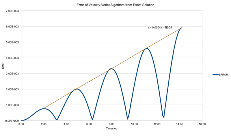
TASK: For the default timestep value, 0.1, estimate the positions of the maxima in the ERROR column as a function of time. Make a plot showing these values as a function of time, and fit an appropriate function to the data.

It is interesting to note that the total error increases linearly with time, indicating that the errors from previous loops of the verlet algorithm are carried forward with each cycle.

TASK: Experiment with different values of the timestep. What sort of a timestep do you need to use to ensure that the total energy does not change by more than 1% over the course of your "simulation"? Why do you think it is important to monitor the total energy of a physical system when modelling its behaviour numerically?

Here you can see the graph of energy that varies by no more than 1%. This is achieved by a timestep of 0.2. It is important to keep track of physical properties of the system to make sure that the numerical modelling is doing it's job correctly, and that the model is a good approximation of the real physical system.

TASK: For a single Lennard-Jones interaction, $\varphi \left(r\right)=4ϵ(\frac{{\sigma }^{12}}{r^{12}}-\frac{{\sigma }^6}{r^6})$, find the separation, $r_0$, at which the potential energy is zero. What is the force at this separation? Find the equilibrium separation, $r_{eq}$, and work out the well depth $(\varphi \left(r_{eq}\right))$. Evaluate the integrals $\underset{2\sigma }{\overset{\mathrm{\infty }}{\int }}\varphi \left(r\right)\mathrm{d}r,\underset{2.5\sigma }{\overset{\mathrm{\infty }}{\int }}\varphi \left(r\right)\mathrm{d}r$, and $\underset{3\sigma }{\overset{\mathrm{\infty }}{\int }}\varphi \left(r\right)\mathrm{d}r$ when $\sigma =ϵ=1.0.$

The separation bond length at $\varphi (r)=0$ is simply $r_o=\sigma$, as when the two are equal, $\frac{{\sigma }^{12}}{r^{12}}-\frac{{\sigma }^6}{r^6}=0$ .

The equilibrium bond length is $2^{1/6}\sigma =r_{eq}$ from:

$0=-4ϵ(\frac{-12{\sigma }^{12}}{r_{eq}^{13}}+\frac{6{\sigma }^6}{r_{eq}^7})$

$\frac{12{\sigma }^{12}}{r_{eq}^{1}3}=\frac{6{\sigma }^6}{r_{eq}^7}$

$\frac{2{\sigma }^{12}}{{\sigma }^6}=\frac{r_{eq}^{13}}{r_{eq}^7}$

$2{\sigma }^6=r_{eq}^6$

Well Depth at $r_{eq}$:

$\varphi \left(r_{eq}\right)=4ϵ(\frac{{\sigma }^{12}}{r_{eq}^{12}}-\frac{{\sigma }^6}{r_{eq}^6})$

$\varphi \left(r_{eq}\right)=4ϵ(\frac{{\sigma }^{12}}{(2^{1/6}\sigma {)}^{12}}-\frac{{\sigma }^6}{(2^{1/6}\sigma {)}^6})$

$\varphi \left(r_{eq}\right)=4ϵ(\frac{{\sigma }^{12}}{2^2{\sigma }^{12}}-\frac{{\sigma }^6}{2{\sigma }^6})$

$\varphi \left(r_{eq}\right)=4ϵ(\frac{1}{4}-\frac{1}{2})$

$\varphi \left(r_{eq}\right)=-ϵ$

Integrals:

$\underset{2}{\overset{\mathrm{\infty }}{\int }}\varphi \left(r\right)\mathrm{d}r=\underset{2}{\overset{\mathrm{\infty }}{\int }}4(\frac{1}{r^{12}}-\frac{1}{r^6})\mathrm{d}r=4{[\frac{1}{5r^5}-\frac{1}{11r^{11}}]}_2^{\mathrm{\infty }}=-0.0248$

$\underset{2.5}{\overset{\mathrm{\infty }}{\int }}\varphi \left(r\right)\mathrm{d}r=\underset{2.5}{\overset{\mathrm{\infty }}{\int }}4(\frac{1}{r^{12}}-\frac{1}{r^6})\mathrm{d}r=4{[\frac{1}{5r^5}-\frac{1}{11r^{11}}]}_{2.5}^{\mathrm{\infty }}=-0.00817$

$\underset{3}{\overset{\mathrm{\infty }}{\int }}\varphi \left(r\right)\mathrm{d}r=\underset{3}{\overset{\mathrm{\infty }}{\int }}4(\frac{1}{r^{12}}-\frac{1}{r^6})\mathrm{d}r=4{[\frac{1}{5r^5}-\frac{1}{11r^{11}}]}_3^{\mathrm{\infty }}=-0.00329$

TASK: Estimate the number of water molecules in 1ml of water under standard conditions. Estimate the volume of 10000 water molecules under standard conditions.

$3.34*10^{22}$ molecules in 1 mL water. This is knowing that the density of water is 1 g/cm^3, and that 1mL - 1cm^3. Therefore the number of moles is 1/18 = 0.05 mol. Multiply that by avagadro's number and you get the answer.

$3*10^{-}19$ mL water contains 10 000 molecules, from $18*\frac{100000}{6.023*10^{-23}}$ for the number of grams, which is equal to the number of mL.

TASK: Consider an atom at position \left(0.5, 0.5, 0.5\right) in a cubic simulation box which runs from $(0,0,0)$ to $(1,1,1)$. In a single timestep, it moves along the vector $(0.7,0.6,0.2)$. At what point does it end up, after the periodic boundary conditions have been applied?.

After the periodic boundary conditions are applied. the molecule is at (0.2, 0.1, 0.7)

TASK: The Lennard-Jones parameters for argon are $$\begin{gathered} \sigma =0.34\mathrm{n}\mathrm{m},ϵ \\ / \\ {k}_B=120\mathrm{K}. \end{gathered}$$ If the LJ cutoff is $r^{*}=3.2$, what is it in real units? What is the well depth in $$\begin{gathered} {\mathrm{k}\mathrm{J} \\ \mathrm{m}\mathrm{o}\mathrm{l}}^{-1} \end{gathered}$$? What is the reduced temperature $T^{*}=1.5$ in real units?

r* in real units is 1.088 nm from $r^{*}=\frac{r}{\sigma }$

Well depth is $-ϵ$. So the well depth is $-1.66*10^{-24}kJmo{l}^{-1}$ from $ϵ=-120k_B$

T*= 180K in non-reduced units from $T=\frac{ϵT^{*}}{k_B}=120T^{*}$

Equilibration:

TASK: Why do you think giving atoms random starting coordinates causes problems in simulations? Hint: what happens if two atoms happen to be generated close together?

If two atoms are very close together, the repulsive interactions of the potential dominate. If they are too close together, they will repel each other with forces that would not happen in nature. Also, it might also prevent the simulation from working in the first place, if such great repulsions are present, messing up calculations.

TASK: Satisfy yourself that this lattice spacing corresponds to a number density of lattice points of 0.8. Consider instead a face-centred cubic lattice with a lattice point number density of 1.2. What is the side length of the cubic unit cell?

A number density of 0.8 can be obtained by plugging in values into $\frac{N}{V}$. For the simple cubic lattice with one atom per unit cell this is $\frac{1}{1.07722^3}$ which indeed equals 0.8. For an fcc lattice, with 4 atoms per unit cell, we get $(\frac{4}{1.2}{)}^{1/3}$ from rearranging the previous formula. This yields a lattice parameter of 1.49 for the fcc lattice.

TASK: Consider again the face-centred cubic lattice from the previous task. How many atoms would be created by the create_atoms command if you had defined that lattice instead?

If 1000 atoms are created for the simple cubic lattice with one atom per unit cell, 4000 atoms would be created for the fcc lattice as there are 4 atoms per unit cell.

TASK: Using the LAMMPS manual, find the purpose of the following commands in the input script:

mass 1 1.0
pair_style lj/cut 3.0
pair_coeff * * 1.0 1.0

The comment essentially sets the mass for the atoms, and the pairwise potential interactions between the atoms, setting the cutoff at which the interactions exist. Beyond the radius of that cutoff, there will be no interactions between atoms. The pair-coeff part simply applies coefficient to different types of atoms (none here, so both =1).

TASK: Given that we are specifying ${\mathbf{x}}_i\left(0\right)$ and ${\mathbf{v}}_i\left(0\right)$, which integration algorithm are we going to use?

We use the velocity-verlet algorithm with those starting parameters.

TASK: Look at the lines below.

### SPECIFY TIMESTEP ###
variable timestep equal 0.001
variable n_steps equal floor(100/${timestep})
variable n_steps equal floor(100/0.001)
timestep ${timestep}
timestep 0.001

### RUN SIMULATION ###
run ${n_steps}
run 100000

The second line (starting "variable timestep...") tells LAMMPS that if it encounters the text ${timestep} on a subsequent line, it should replace it by the value given. In this case, the value ${timestep} is always replaced by 0.001. In light of this, what do you think the purpose of these lines is? Why not just write:

timestep 0.001
run 100000

The lines put the timestep into a variable which can be used later to calculate properties. If the bottom version is used, then the timestep is not saved into a variable, the system runs and never outputs any timestep. A lot of calculations would therefore not be feasible.

TASK: make plots of the energy, temperature, and pressure, against time for the 0.001 timestep experiment (attach a picture to your report). Does the simulation reach equilibrium? How long does this take? When you have done this, make a single plot which shows the energy versus time for all of the timesteps (again, attach a picture to your report). Choosing a timestep is a balancing act: the shorter the timestep, the more accurately the results of your simulation will reflect the physical reality; short timesteps, however, mean that the same number of simulation steps cover a shorter amount of actual time, and this is very unhelpful if the process you want to study requires observation over a long time. Of the five timesteps that you used, which is the largest to give acceptable results? Which one of the five is a particularly bad choice? Why?

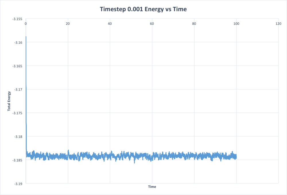
In the graph above, where the total energy vs time is plotted for the simulation with the timestep of 0.001, it can be clearly seen that an equilibrium is reached at relatively low times. This can be seen by the fact that a constant energy is reached, around which the system oscillates. If one then looks at how the total energy varies with differing timestep, the following plot results.

This plot shows that the worst timestep to use is indeed 0.015, as the total energy does not reach a constant value- it diverges rather than converging. This definitely does not represent physical reality. 0.0075 and 0.01 are decent approximations, but the larger timestep leads to a higher total energy value, meaning that while the system is moderately representative of the physical system, it is not entirely accurate. The highest timestep that still gives results that as are good as 0.001 is actually 0.0025, which comes to the same, or very similar total energy as the timestep 0.001.

Running Simulations under Specific Conditions:

TASK: Choose 5 temperatures (above the critical temperature T^* = 1.5), and two pressures (you can get a good idea of what a reasonable pressure is in Lennard-Jones units by looking at the average pressure of your simulations from the last section). This gives ten phase points — five temperatures at each pressure. Create 10 copies of npt.in, and modify each to run a simulation at one of your chosen \left(p, T\right) points. You should be able to use the results of the previous section to choose a timestep. Submit these ten jobs to the HPC portal. While you wait for them to finish, you should read the next section.

The temperatures used were 1.5, 1.7, 1.9, 2.1, and 2.3, while the pressures used were 2 and 3.

There were two timesteps I considered using for the simulation. 0.001 was obviously the most accurate, though 0.0025 was very similar. In the end, I decided that I would run the more accurate simulation, however if I were to run much longer simulations, I would go for the 0.0025 timestep to save more time.

TASK: We need to choose $\gamma$ so that the temperature is correct $T=\mathfrak{𝔗}$ if we multiply every velocity $\gamma$. We can write two equations:

$E_K=\frac{3}{2}N{k}_{B}T$

$\frac{1}{2}\sum _i{m}_i{v}_i^2=\frac{3}{2}N{k}_{B}T$

Solve these to determine $\gamma$.

$\frac{1}{2}\sum _i{m}_i(\gamma v_i{)}^2=\frac{3}{2}N{k}_B\mathfrak{𝔗}$

$\frac{1}{2}\sum _i{m}_i{v}_i^2=\frac{3}{2}N{k}_{B}T$

$\frac{\frac{1}{2}\sum _i{m}_i(\gamma v_i{)}^2}{\frac{1}{2}\sum _i{m}_i{v}_i^2}=\frac{\frac{3}{2}N{k}_B\mathfrak{𝔗}}{\frac{3}{2}N{k}_{B}T}$

$\frac{{\gamma }^2\frac{1}{2}\sum _i{m}_i{v}_i^2}{\frac{1}{2}\sum _i{m}_i{v}_i^2}=\frac{\frac{3}{2}N{k}_B\mathfrak{𝔗}}{\frac{3}{2}N{k}_{B}T}$

$\gamma =\sqrt{(}\mathfrak{𝔗}/T)$

TASK: Use the manual page to find out the importance of the three numbers 100 1000 100000. How often will values of the temperature, etc., be sampled for the average? How many measurements contribute to the average? Looking to the following line, how much time will you simulate?

Every 100 timesteps the temperature will be sampled for the average

1000 measurements contribute to the average

100 000 steps will be simulated which is 10000 * timestep = time.

TASK: When your simulations have finished, download the log files as before. At the end of the log file, LAMMPS will output the values and errors for the pressure, temperature, and density $\left(\frac{N}{V}\right)$. Use software of your choice to plot the density as a function of temperature for both of the pressures that you simulated. Your graph(s) should include error bars in both the x and y directions. You should also include a line corresponding to the density predicted by the ideal gas law at that pressure. Is your simulated density lower or higher? Justify this. Does the discrepancy increase or decrease with pressure?

In order to put ideal gas curves on the graph, the ideal gas equation has to be rearranged then converted into reduced units.

$\frac{P}{k_{B}T}=\frac{N}{V}=\rho$

Here P, T, and $\rho$ both have to be converted into P*, T*, and ${\rho }^{*}$

$T^{*}=\frac{k_{B}T}{ϵ}$

$P^{*}=\frac{\sum E^{*}}{\sum V^{*}}=\frac{\frac{E}{ϵ}}{(\frac{r}{\sigma }{)}^3}$

$P^{*}=\frac{E}{V}\frac{{\sigma }^3}{ϵ}$

${\rho }^{*}=\frac{P^{*}}{T^{*}}=\frac{P^{*}}{{\sigma }^3{T}^{*}}$

From here, the values for pressure and temperature in reduced units are fed into the equation, and the density in reduced units is produced. These curves can be seen on the graph below, on the same plot as the simulation density/temperature variation.

At lower temperatures the discrepancy is larger, though the errors of the points at lower temperatures are smaller, presumably due to less thermal motion. to the fact that at lower tem Density of the ideal gas equivalent is higher because it does not take into account any interactions or repulsion so the particles can come much closer to each other and stay close. Since there is a set starting lattice for the simulations, the density is related to this starting setup. If there are no repulsive forces they can stay close to each other, even when moving more rapidly. . Physically it makes that the density decreases with temperature, due to the concept of thermal expansion, and what we intuitively know about liquids. (We are going to ignore the case of water- this simulation does not take into account the weird and wonderful world of water, this is a simple liquid after all). In both cases the density is decreasing due to increasing entropy of the system, and with greater entropy the system will want to occupy more space, and hence lower the density. Another cause for the discrepancy at low T is that the expression used for density, derived from the ideal gas equation, has T in the denominator. Therefore as T approaches zero, the density will tend to infinity. WIth the Lennard-Jones liquid, however, there is the repulsive term that prevents the atoms from getting too close, and keeping the density relatively low.

Heat Capacities

TASK: As in the last section, you need to run simulations at ten phase points. In this section, we will be in density-temperature $({\rho }^{*},T^{*})$ phase space, rather than pressure-temperature phase space. The two densities required at 0.2 and 0.8, and the temperature range is 2.0, 2.2, 2.4, 2.6, 2.8. Plot C_V/V as a function of temperature, where V is the volume of the simulation cell, for both of your densities (on the same graph). Is the trend the one you would expect? Attach an example of one of your input scripts to your report.

The heat capacities from the file output are given by $C_V^{*}=N^2*\frac{var[E^{*}]}{(T^{*}{)}^2}$ In order to get the heat capacity per unit volume, the value of heat capacity that is output by the simulation must be multiplied by $\frac{{\rho }^{*}}{N}$, where N is 3374 atoms. The results are plotted in the chart below.

Here you can see that heat capacity is decreasing with temperature. Going from basic thermodynamic principles $C_v=\frac{dQ}{dT}$. Assuming that Q is independent of T, we would get a constant value for the heat capacity, one that does not depend on temperature. However, there is a clear variation of heat capacity with temperature, as it decreases with increasing temperature. This could be considered an example of a Schottky anomaly, where the heat capacity decreases after it reaches a peak at low energies. This is indicative of a system with two energy levels that have an energy spacing similar to that of low temperatures, and once the temperature increases past that of the energy separation of the states, the heat capacity decreases as the levels are equally occupied, and an increase in temperature has little to no impact on the entropy. As the heat capacity is related to the entropy through temperature, ($S=\underset{0}{\overset{T}{\int }}\left(\frac{C_v}{T}\right)dT$) this results in a decrease in the heat capacity.

Example input file here

Structural properties and the radial distribution function

TASK: perform simulations of the Lennard-Jones system in the three phases. When each is complete, download the trajectory and calculate g(r) and $\int g(r)\mathrm{d}r$. Plot the RDFs for the three systems on the same axes, and attach a copy to your report. Discuss qualitatively the differences between the three RDFs, and what this tells you about the structure of the system in each phase. In the solid case, illustrate which lattice sites the first three peaks correspond to. What is the lattice spacing? What is the coordination number for each of the first three peaks?

The first three peaks of the solid RDF correspond to the three nearest neighbors, which can be see in the image adjacent. The first peak should represent $\frac{a}{\sqrt{2}}$ where a is the lattice parameter. For the solid state, the lattice parameter is 1.493 (taken from the output file). Plugging this into the previous formula, this says that the nearest neighbor should be at r=1.05. Indeed, the first peak for the solid RDF is at just over 1. Only 1.025 rather than 1.05, but then again there is vibrational energy in the lattice, which is why the peaks are broad rather than essentially delta functions. The next nearest neighbor should be at $r=a$. Once again, this is indeed the case, as the second peak is at 1.475 (close to 1.493!). The third peak should be at 1.828 ($\sqrt{\frac{3}{2}}a$), and indeed the third peak is at r=1.825. So the RDF very clearly and accurately shows the lattice parameter and the nearest neighbors in r.

Circled is the reference point. Orange is the nearest neighbor, green the next-nearest, and red the third-nearest

As you can see on the graph, there are three very distinct RDFs, one for each phase. The RDF for the gas phase shows a single peak at just over 1, that decays with little to no fluctuation quite quickly. Liquid peaks slightly earlier and has far more fluctuations, which are more fluid than the fluctuations of solid. The solid RDF has much more choppy peaks that are also at slightly lower r. This is because the location of the next nearest neighbors are much more well-defined, at a better-defined value of r in solids. With liquid the curves are broader due to the lack of long-range order- they look more like the curves you would see for the radial distribution function of an atomic orbital. The breadth of the curve says that there is probably a liquid molecule in that range of r. Since a gas is so disperse there are no peaks.

The coordination number of the first three peaks for the solid RDF can be found by looking at the data from the running integral, as the area under g(r) represents the number of nearest neighbors, as g(r) is a function of density in space. The coordination number for the nearest neighbor is 12, which can be seen from the running integral value of 12.01. The next peak has an integral of 6 (18.4-12.01), while the final peak has the integration value of 24 again (23.86, 42.26-18.4). When picturing the crystal lattice, this makes geometrical sense. So the coordination number of the first peak is 12, for the second peak it's 6, and for the third it's 24. The data was taken from the files output by the VMD.

Dynamical properties and the diffusion coefficient

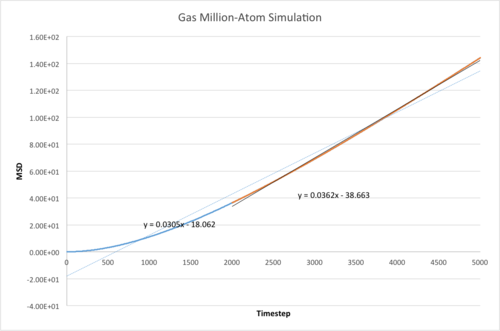
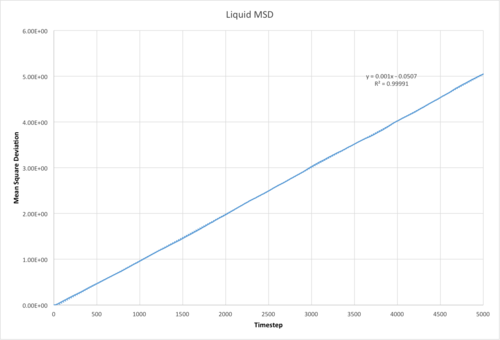
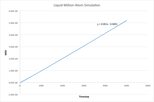
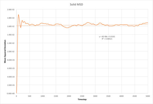
TASK: make a plot for each of your simulations (solid, liquid, and gas), showing the mean squared displacement (the "total" MSD) as a function of timestep. Are these as you would expect? Estimate D in each case. Be careful with the units! Repeat this procedure for the MSD data that you were given from the one million atom simulations.

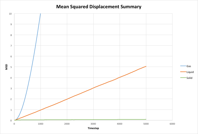
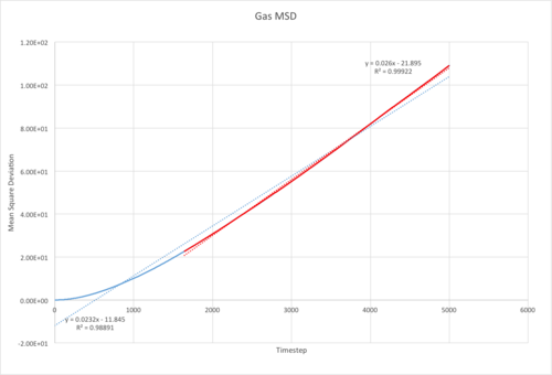
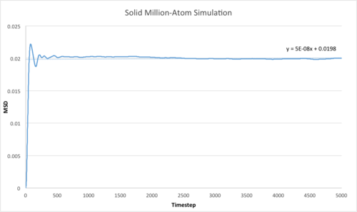
Above is the general MSD plot, which shows very clearly that the slopes of the MSD plots vary immensely from one phase to the next. Below are the separate plots for the MSD for each phase, and for my simulation and the million-atoms simulation. They are quite similar, however the solid million-atom simulation is a bit smoother. This is probably because the thermal motion of all of the atoms tend to cancel each other out in larger values, as is central in statistical thermodynamics (ergodicity). If you enlarge the images, you can see the lines of best fit used to calculate the diffusion coefficient. Note that for the gas phase, a line of best fit is only fitted to the linear portion of the graph, and took the line of best fit for that. I included the other line of best fit and Rsquared values to show which line of best fit had a better fit. The line of best fit is important for the averaged part of the mean squared deviation.

Since all of the values have the same arbitrary units, there does not need to be any kind of unit manipulation, and the values can simply be compared.

Using $D=\frac{1}{6}\frac{\partial ⟨r^2\left(t\right)⟩}{\partial t}$, I got the following values for D from the gradient of the line once a visible equilibrium had roughly been met:

	Simulation	Million
Gas	0.0043	0.00603
Liquid	0.00016	0.00016
Solid	$1x10^{-8}$	$8.3x10^{-9}$

These values make sense logically. Gases and liquids are subject to thermal motion, and we know intuitively that they diffuse- otherwise a lot of our chemistry would be limited. This means that they will have non-zero values for D, which is what we observe. Since solids are locked into their lattices, they will not exhibit any diffusion. The values for D we get here for the solids are definitely very very close to 0. In fact, the reason why it is non-zero is probably that the first section of the graph, where it was still equilibrating, was included, as well as the general fluctuations due to thermal motion. In a real crystal, the diffusion coefficient would be non-zero, due to defects in the crystal that can diffuse (slowly!) through the lattice. A gas has a higher diffusion constant than a liquid as the particles are much further apart and can move freely without any major interactions, and can therefore diffuse through space more easily. Due to the proximity of other particles in the liquid phase that interact more strongly, liquids have lower diffusion. Entropically this also makes sense; phases with higher entropy will diffuse more rapidly due to the greater number of accessible microstates of a diffuse phase.

The fact that the million-atoms simulations are not hugely different to the smaller simulations indicates that it is possible to compute smaller systems and apply results to larger systems as needed to save computational power and time. The values for the diffusion coefficients are a bit more extreme for the million-atom simulation, highlighting their differences a bit more, but only minorly.

TASK: In the theoretical section at the beginning, the equation for the evolution of the position of a 1D harmonic oscillator as a function of time was given. Using this, evaluate the normalised velocity autocorrelation function for a 1D harmonic oscillator (it is analytic!):

$C\left(\tau \right)=\frac{\underset{-\mathrm{\infty }}{\overset{\mathrm{\infty }}{\int }}v(t)v(t+\tau )\mathrm{d}t}{\underset{-\mathrm{\infty }}{\overset{\mathrm{\infty }}{\int }}{v}^2(t)\mathrm{d}t}$

Be sure to show your working in your writeup. On the same graph, with x range 0 to 500, plot C\left(\tau\right) with \omega = 1/2\pi and the VACFs from your liquid and solid simulations. What do the minima in the VACFs for the liquid and solid system represent? Discuss the origin of the differences between the liquid and solid VACFs. The harmonic oscillator VACF is very different to the Lennard Jones solid and liquid. Why is this? Attach a copy of your plot to your writeup.

$C(\tau )=\frac{\underset{-\mathrm{\infty }}{\overset{\mathrm{\infty }}{\int }}v\left(t\right)v(t+\tau )\mathrm{d}t}{\underset{-\mathrm{\infty }}{\overset{\mathrm{\infty }}{\int }}{v}^2\left(t\right)\mathrm{d}t}$

$x(t)=A\cos (\omega t+\varphi )$

$v(t)=-A\omega \sin (\omega t+\varphi )$

$v(t+\tau )=-A\omega \sin (\omega (t+\tau )+\varphi )$

$C(\tau )=\frac{\underset{-\mathrm{\infty }}{\overset{\mathrm{\infty }}{\int }}-A\omega \sin (\omega t+\varphi )*-A\omega \sin (\omega (t+\tau )+\varphi )\mathrm{d}t}{\underset{-\mathrm{\infty }}{\overset{\mathrm{\infty }}{\int }}(-A\omega {)}^2{\sin }^2(\omega t+\varphi )\mathrm{d}t}$

$C(\tau )=\frac{(A\omega {)}^2\underset{-\mathrm{\infty }}{\overset{\mathrm{\infty }}{\int }}\sin (\omega t+\varphi )\sin (\omega \tau +\varphi )\mathrm{d}t}{(A\omega {)}^2\underset{-\mathrm{\infty }}{\overset{\mathrm{\infty }}{\int }}si{n}^2(\omega t+\varphi )\mathrm{d}t}$

Next we set

$\alpha =\omega t,\beta =\omega \tau$

$C(\tau )=\frac{\underset{-\mathrm{\infty }}{\overset{\mathrm{\infty }}{\int }}\sin (\alpha )\sin (\alpha +\beta )\mathrm{d}\alpha }{\underset{-\mathrm{\infty }}{\overset{\mathrm{\infty }}{\int }}{\sin }^2(\alpha )\mathrm{d}\alpha }$

The next step is to use the trig identity $\sin (\alpha +\beta )=\sin \alpha \cos \beta +\cos \alpha \sin \beta$:

$C(\tau )=\frac{\underset{-\mathrm{\infty }}{\overset{\mathrm{\infty }}{\int }}{\sin }^2\alpha \cos \beta +\sin \alpha \cos \alpha \sin \beta \mathrm{d}\alpha }{\underset{-\mathrm{\infty }}{\overset{\mathrm{\infty }}{\int }}{\sin }^2(\alpha )\mathrm{d}\alpha }$

$$\begin{gathered} C(\tau )=\frac{\underset{-\mathrm{\infty }}{\overset{\mathrm{\infty }}{\int }}{\sin }^2\alpha \cos \beta \mathrm{d}\alpha }{\underset{-\mathrm{\infty }}{\overset{\mathrm{\infty }}{\int }}{\sin }^2(\alpha )\mathrm{d}\alpha }+\frac{\underset{-\mathrm{\infty }}{\overset{\mathrm{\infty }}{\int }} \\ \sin \alpha \cos \alpha \sin \beta \mathrm{d}\alpha }{\underset{-\mathrm{\infty }}{\overset{\mathrm{\infty }}{\int }}{\sin }^2(\alpha )\mathrm{d}\alpha } \end{gathered}$$

$$\begin{gathered} C(\tau )=\cos \beta +\frac{\sin \beta \underset{-\mathrm{\infty }}{\overset{\mathrm{\infty }}{\int }} \\ \sin \alpha \cos \alpha \mathrm{d}\alpha }{\underset{-\mathrm{\infty }}{\overset{\mathrm{\infty }}{\int }}{\sin }^2(\alpha )\mathrm{d}\alpha } \end{gathered}$$

Then use the trig identity $\frac{1}{2}\sin x\cos x=\sin (2x)$

$$\begin{gathered} C(\tau )=\frac{\cos \beta \underset{-\mathrm{\infty }}{\overset{\mathrm{\infty }}{\int }}{\sin }^{}\alpha \mathrm{d}\alpha }{\underset{-\mathrm{\infty }}{\overset{\mathrm{\infty }}{\int }}{\sin }^2(\alpha )\mathrm{d}\alpha })+\frac{2\sin \beta \underset{-\mathrm{\infty }}{\overset{\mathrm{\infty }}{\int }} \\ \sin (2\alpha )\mathrm{d}\alpha }{\underset{-\mathrm{\infty }}{\overset{\mathrm{\infty }}{\int }}{\sin }^2(\alpha )\mathrm{d}\alpha } \end{gathered}$$

Here the second term falls away due to the odd nature of $\sin (2\alpha )$, rendering it's integral equal to zero. (If you look at it theoretically, the integral diverges). The integral of sin^2 alpha cancels out in the first term, leaving the velocity autocorrelation function as $C(\tau )=\cos (\beta )=\cos (\omega \tau )$.

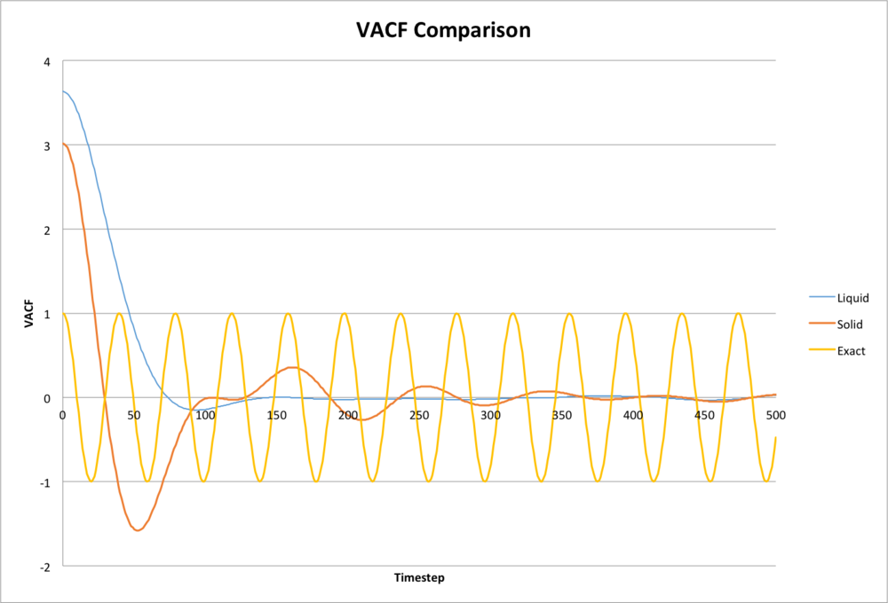
Clearly there is a difference between the solution for the harmonic oscillator VACF and the Lennard-Jones potential used for the simulations. Most notable is the fact that the VACF starts much higher, and falls away quite quickly. The liquid VACF also doesn't even undergo a full oscillation, but dies down quite quickly after a broad peak. The solid VACF has more evident but damped oscillations due to more rigid long-range order. Since the positions of atoms are better-defined, the oscillations are more similar to the harmonic oscillator than the liquid. The damping of the "oscillations" of the solid and liquid are due to collisions and interactions between particles. The harmonic oscillator approximation only holds if there are no collisions or only around the absolute equilibrium of the system, which is definitely not the case. Also the Lennard Jones potential is anharmonic, so as things interact and move around, that anharmonicity will cause a change.

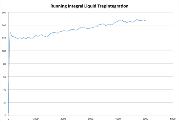
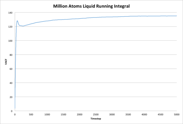
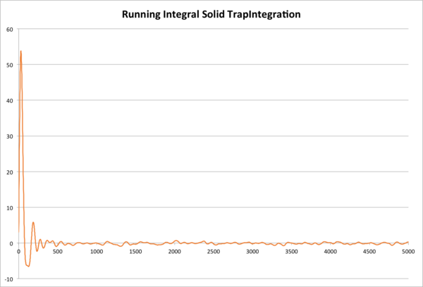
TASK: Use the trapezium rule to approximate the integral under the velocity autocorrelation function for the solid, liquid, and gas, and use these values to estimate D in each case. You should make a plot of the running integral in each case. Are they as you expect? Repeat this procedure for the VACF data that you were given from the one million atom simulations. What do you think is the largest source of error in your estimates of D from the VACF?

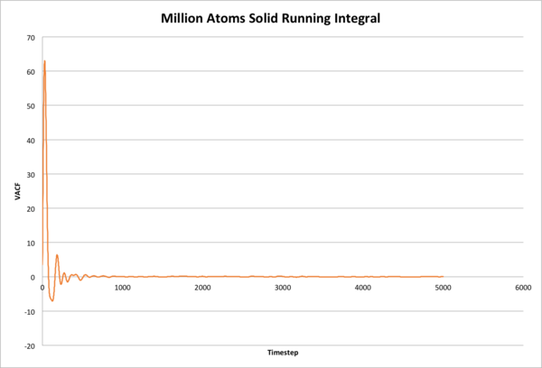
Using the final running integral value for each TrapIntegration plot, I calculated the following values for D using $D=\frac{1}{3}\underset{0}{\overset{\mathrm{\infty }}{\int }}\mathrm{d}\tau ⟨\mathbf{v}\left(0\right)\cdot \mathbf{v}\left(\tau \right)⟩$:

	Simulation	Million
Liquid	48.9444	45.0457
Solid	0.09405	0.02276

These are rather noticeably different to the values achieved from the MSD above, though the same general pattern holds: the liquid simulation has a much much higher value for the diffusion coefficient than the solid. The gas graphs were not included (because they were not requested) due to the fact that in the timespan of the simulation, the gas never reached a plateau, the graph of the running integral was more of a gentle curve upwards, slope decreasing but definitely not plateauing in the timeframe of the simulation. This is probably due to the highly diffuse nature of gases compared to liquids and solids.

The limitations of the VACF lie in the fact that it assumes that the velocity remains the same regardless of collision, while in reality, collisions frequently change the velocity of particles. This may be why the values are so different to the values from the mean square deviation method of calculation. Another major error of this method is the fact that it uses the trapezium rule, a rather crude approximation, to find the numerical integral of the VACF. Also, as the timesteps are given as 1,2,3,.. etc, there is no opportunity for the value of h, or the width of the trapezium, to be reduced further, which would allow for a more accurate calculation. Perhaps using the actual value of time rather than timestep would allow for more precise measurement, though that would bring units into the fray.