Rep:Mod:physY3LAWCHCOMP

Introduction

Computational chemistry is a useful and powerful tool when it comes to analysing the finer details of chemical reactions that would be practically difficult (or even impossible) to measure or observe in a laboratory setting, and so it has an increasingly important role in both research (i.e. pharmaceuticals) and understanding chemical theory. In this module, the aim is to do the latter by investigating how two pericyclic reactions proceed (Cope rearrangement and Diels-Alder Cycloaddition). The transition state structures involved can be obtained using molecular orbital based calculations to determine the potential energy surface of the molecule, where any maximum points will correspond to a transition state. The GaussView and Gaussian software packages are used to optimise the structures of the reactants, products and transition states, to calculate energies and vibrational frequencies and to visualise the frontier orbitals and reaction co-ordinates in an attempt to understand the reaction mechanism, energetics and any aspects of selectivity.

Cope Rearrangement

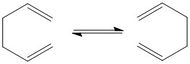
Fig. 1: Cope rearrangement of 1,5-hexadiene

The [3,3] Cope sigmatropic rearrangement of 1,5-hexadiene is investigated below. Part 1 involves optimising the structures of the reactant and product to determine which conformation is lowest in energy and thus adopted in reality. 1,5-hexadiene is able to adopt both anti and gauche conformations, and the energies of these different individual conformers can be computed using the Hartree Fock (HF) method and 3-21G basis set. Once the minimum energy structure is determined, a frequency calculation can be carried out to yield a more accurate estimate of the energy of the molecule which can subsequently be compared with literature values to evaluate the accuracy of the prediction under this method and basis set. Part 2 involves locating the structure of the 6-membered transition states using three different methods (Hessian, Frozen Co-ordinate, QST2) and then to calculate the energy barrier for the forward reaction shown in Fig. 1. This will be carried out twice using two different basis sets: first with the HF/3-21G and then with the DFT B3LYP/6-31G set, which is based on quantum mechanics.

Part 1: Optimising Reactants and Products

As mentioned briefly above, 1,5-hexadiene can adopt both anti conformations (where the torsion angle between the two double bonds is approximately 180 °) and gauche conformation (where the torsion angle between the double bonds is 60 °). Below in Table 1 are examples of both conformations- the structures were drawn on GaussView and optimised using the HF/3-21G method and basis set.

Log anti 1 Log gauche 1

Table 1: Examples of *anti* and *gauche* 1,5-hexadiene conformations
Conformation:	Newman Projection:*	Structure:	Point Group:	Energy/ a.u.:
1 (Anti)			Ci	-231.68539585
2 (Gauche)			C2	-231.68771610

*Note: The Newman projections drawn are from the perspective of looking down the C3-C4 bond.

Normally, it would be assumed that the anti conformation would be more stable (i.e. lower in energy) than the gauche conformation (as seen in n-butane, for example) as the two 'bulky' vinyl groups are the furthest distance they can be apart (180 °). However, the calculated energies of the two conformations indicate that the gauche structure is, in fact, slightly lower in energy than the anti structure, and thus more stable. The difference between the two predicted values = 0.00232025 a.u. which corresponds approximately to a 6 kJmol^-1 barrier to rotation between these two particular conformations. Therefore, there must be favourable stereoelectronic interactions between the two groups that leads to the gauche form being preferentially adopted over the anti form of 1,5-hexadiene.

It is important to remember that there are three C-C bonds which can rotate, and therefore the substituents can also be described as being anti or gauche with respect of each of these bonds. This leads to 27 theoretically possible conformations for 1.5-hexadiene, but only 10 of these are energetically distinct.^[1] In the case of the gauche structure shown in Table 1, it can be seen that the two vinyl groups are gauche with respect to the central C-C bond, but in fact the two large groups are eclipsed (torsion angle = 0 °) with respect to the other two C-C bonds (see Table 2).

Table 2: Diagrams illustrating that the *gauche* conformation in Table 1 is *gauche* with respect to C3-C4
View along C2-C3:	View along C3-C4:	View along C4-C5:

Eclipsed	Gauche	Eclipsed

This would indicate that there are possible lower energy conformations of 1,5-hexadiene that should have torsion angles > 0 ° with respect to all three rotating C-C bonds. The minimum structure was found to be that shown in Table 3:

Log gauche lowestenergy

Table 3: Predicted minimum energy conformation of 1,5-hexadiene
Conformation:	Structure:	Point Group:	Energy/ a.u.:
3 (Gauche)		C1	-231.69266121

Looking down each of the bonds, it can be seen that the torsion angle between the large groups is now 120 ° rather than 0 °, which is sterically more favourable.

Table 4: Diagrams illustrating the torsion angles in the lowest energy *gauche* structure
View along C2-C3:	View along C3-C4:	View along C4-C5:

Clinal	Gauche	Clinal

The structures drawn above can be identified by comparison with those shown in Appendix 1 of the tutorial wiki page. Structure 1 corresponds to anti2; structure 2 corresponds to gauche, and the lowest energy structure 3 corresponds to gauche3. The energies of the two gauche conformations above closely match those provided in the Appendix. However, although the anti conformation in Table 1 has the same point group (Ci) as that of anti2, the energy values of both structures are markedly different- the structure in Table 1 has a value of -231.68539585 a.u. compared to the appendix structure which has an energy = -231.69254 a. u., which gives rise to a difference of 0.00714415 a.u. (approximately 18 kJmol^-1 !). Taking a closer look at the exact structures depicted in the images, it appears that the difference in energy may be associated with the position of the hydrogen atoms- in the Appendix image, the hydrogen atoms attached to the C=C double bond face out of the plane of the molecules and the C-C hydrogen atoms lie in the plane; the structure in Table 1 implies the reverse, and is found be to higher in energy. In order to minimise the energy of the Ci conformer above, the hydrogen atoms were re-orientated to be in the positions implied in the anti2 conformation:

Log re-drawn structure anti2

Table 5: Redrawn and re-optimised structure of *anti2* 1,5-hexadiene
Conformation:	Structure:	Point Group:	Energy/ a.u.:
anti2		Ci	-231.69253529

This reorganisation of the hydrogen atoms is of a lower energy and matches the value quoted in the Appendix much more closely. This redrawn anti2 configuration was then re-optimised using the quantum mechanical DFT B3LYP/6-31G method and basis set.

Log B3LYP/6-31G OPT+FREQ anti2

Table 6: Structure of the DFT B3LYP/6-31G optimised *anti2* 1,5-hexadiene
Conformation:	Structure:	Point Group:	Energy/ a.u.:
anti2		Ci	-234.61170222

It is expected that the quantum mechanical method and basis set would generate results that align more accurately with experimentally determined results. Optimising with a higher basis set leads only to minimal changes in the geometry of the molecule- a comparison of some of the geometric parameters is shown below in Table 6. Experimentally determined values for the bonds and angles present in 1,5-hexadiene obtained by electron diffraction are also included for comparison.^[2] The DFT B3LYP/6-31G optimised structure is found to agree slightly better with experimental values except for the bond angle, in which the HF/3-21G is shown to be closer to the observed value.

Table 7: Geometric comparison of the HF/3-21G and DFT B3LYP/6-31G
Model and Basis Set:	HF/3-21G	DFT B3LYP/6-31G	Experimental data
Labelled Structure:
C=C Bond Length/ Å:	1.31616	1.33350	1.340 ± 0.003
C3-C4 Bond Length/ Å:	1.55291	1.54813	1.538 ± 0.027
C2-C3 and C4-C5 Bond Length/ Å:	1.50890	1.50416	1.508 ± 0.012
C2-C3-C4 and C3-C4-C5 angle/ °:	111.348	112.670	111.5 ± 0.900

A frequency calculation was then carried out on the DFT B3LYP/6-31G optimised structure from which the predicted IR spectrum and vibrational modes of the molecule can be visualised. As an example, the calculated IR spectrum of anti2 1,5-hexadiene is shown in Fig. 1 below. The frequency calculation also computes some thermochemical data, most importantly some corrections to the energy of the molecule which can be found in the .log output file (shown in the text box below). These corrections become of importance when comparing to values found in literature- for example, the 'Sum of electronic and zero-point energies' takes into account the vibrational zero point energy and is taken at 0 K whereas the 'Sum of electronic and thermal energies' is the energy of the molecule at room temperature and pressure (298.15 K and 1 atm). The values given below are from the log file of the DFT B3LYP/6-31G optimised anti2 1,5-hexadiene molecule and will be needed later when calculating the activation energies of the transition states in this rearrangement.

 Sum of electronic and zero-point Energies=           -234.469243
 Sum of electronic and thermal Energies=              -234.461877
 Sum of electronic and thermal Enthalpies=            -234.460933
 Sum of electronic and thermal Free Energies=         -234.500889

Part 2a: Optimising the 'Chair' Transition State

The first step towards drawing the transition state structures involves optimising a delocalised allyl fragment to a minimum with the HF/3-21G method and basis set. Once this is completed, two of these allyl fragments are put together with the correct symmetry as shown in Appendix 2 of the tutorial wiki page to give a 'guessed' chair transition state structure which is shown on the right in Fig. 2 (C2h symmetry was imposed on the molecule and the distance between the terminal carbons of the allyl fragments set constant to an initial value of 2.20 Å). Presented in this section are two methods of optimising transition states- the Normal Hessian method and the frozen co-ordinate method (a third alternative will be presented when carrying out the calculations for the 'Boat' transition state).

To optimise this 'guessed' chair transition state using the normal Hessian method, the optimisation calculation on GaussView can be modified slightly so that the optimisation is set to 'transition state (Berny)' rather than the minimum. The 'force constants' option was set to be calculated once and the keyword 'noeigen' was added so that the calculation does not terminate upon detecting imaginary frequencies (which are needed later). Optimisations were carried out first using HF/3-21G method and basis set then re-optimised using DFT B3LYP/6-31G method and basis set.

Table 8: Optimisation results of the guessed chair transition state (Normal Hessian Method)
Method and Basis Set:	Structure and Summary:	Point Group:	Energy/ a.u.:	Distance between terminal allyl carbons/ Å:
HF/3-21G		C2h	-231.61932247	2.02055
DFT B3LYP/6-31G		C2h	-234.50546906	2.03586

There are two pieces of evidence that can be used to confirm that these are transition state structure- the first is to compare these energy values to those calculated previously for 1,5-hexadiene- the transition state should take a higher energy value than the optimised reactant or product.

Table 9: Electronic energies of the chair transition states
Model and Basis Set:	HF/3-21G	DFT B3LYP/6-31G
Electronic Energy of Chair TS/ a.u.:	-231.61932247	-234.50546906
Electronic Energy of optimised 1,5-hexadiene/ a.u.:	-231.69253529	-234.61170222
ΔE_elec/ a.u.:	0.07321282	0.10623316

A second way of determining that this is a transition state is by seeing whether there is one single imaginary frequency present in the vibration analysis- imaginary frequencies are negative frequency values, and because frequency ∝ (force constant)^1/2, this implies that the force constant will be a negative value. The force constant is also equal to the second derivative of the potential energy, and a negative value for the second derivative implies that the turning point on the potential energy surface is a maximum, which is expected for a transition state. The animation should also be the vibration that leads to formation of the product. The imaginary frequency results and animations are shown below for the two methods and basis sets described above.

Table 10: Imaginary frequency of the 1,5-hexadiene chair TS (Hessian method)
Method and Basis Set:	Animation:	Frequency/ cm^-1:
HF/3-21G		-817.93
DFT B3LYP/6-31G		-561.98

The second optimisation method is the frozen co-ordinate method, which involves using the 'redundant co-ordinates' editing option and optimising the transition state twice to a minimum. The redundant co-ordinates are modified so that the distance between the terminal carbons of the allyl groups is frozen (i.e. kept constant) at 2.20 Å during the initial optimisation whilst the rest of the molecule is minimised. During the set-up for the calculation, the keyword 'Opt=ModRedundant' must be present for this to work. Before the second optimisation, the co-ordinates are modified on the checkpoint file so that the 'Derivative' option is selected instead of 'Freeze Co-ordinate'- by differentiating at the reaction co-ordinate, it is possible to obtain a good estimate for the transition state structure and parameters without carrying out a full Hessian calculation, and this may be seen as a viable alternative when more complex molecules are being computationally analysed and the Hessian method may require a long calculation time. The results for the optimisation of the guessed chair transition state structure are shown for the two methods and basis sets in Table 11 and the imaginary frequency results shown in Table 12:

Table 11: Optimisation results of the guessed chair transition state (Frozen Co-ordinate Method)
Method and Basis Set:	Structure and Summary:	Point Group:	Energy/ a.u.:	Distance between terminal allyl carbons/ Å:
HF/3-21G		C2	-231.61932194	2.02052 & 2.01827
DFT B3LYP/6-31G		C2	-234.50546895	2.03683 & 2.03678

Table 12: Imaginary frequency result of 1,5-hexadiene chair TS
Method and Basis Set:	Animation:	Frequency/ cm^-1:
HF/3-21G		-817.98
DFT B3LYP/6-31G		-561.73

Here, it can be seen that this 'frozen co-ordinate' method yields relatively accurate results, and the energies and bond lengths are similar to those calculated using the Hessian method. The distinct difference between the two methods is that the resultant point groups are different- the Hessian gives C2h, which is the expected result, whereas this method gives C2. Also, this transition state is no longer 'symmetrical' as the terminal C-C distances are different values whereas only one value was seen with the Hessian method. The imaginary frequencies occur with similar magnitude to those calculated in the first method.

Part 2b: Optimising the 'Boat' Transition State

The 'boat' is another structure that can be adopted by the transition state, and it is expected to be higher in energy than the chair form (as found for cyclohexane). To optimise this transition state structure, the QST2 method is used, which essentially tries to find the transition state structure as an interpolation between the reactant and product. The first step, therefore, is to create a file with both the product and reactant present in the same window (for this exercise the HF/3-21G optimised anti2 conformation of 1,5-hexadiene was chosen to start with). Next, the atoms are labelled by editing the 'atom list' so that both the reactant and product are numbered in the same way as seen in Fig. 3. A Gaussian calculation can then be set up where the 'opt+freq' option is selected, and the structure allowed to optimise to a 'TS(QST2)', but the results do not show a boat transition state- in fact the optimised structure looks more like a chair.

To obtain the boat transition state, the structures of the reactant and product have to be modified slightly so that the reactant and product resemble a more 'boat-like' structure: i) the dihedral angle C2-C3-C4-C5 was set to be 0 ° and ii) the inside angles C2-C3-C4 and C3-C4-C5 were set to be 100 °. The optimisation to the TS(QST2) was then carried out using both methods and basis sets and the results are shown in Table 13.

Table 13: Optimisation results of the boat transition state (QST2 Method)
Method and Basis Set:	Structure and Summary:	Point Group:	Energy/ a.u.:
HF/3-21G		CS	-231.60280206
DFT B3LYP/6-31G		CS	-234.49288710

Table 14: Imaginary vibrational modes of 1,5-hexadiene chair TS
Method and Basis Set:	Animation:	Frequency/ cm^-1:
HF/3-21G		-839.87
DFT B3LYP/6-31G		-510.35

Part 2c: Intrinsic Reaction Co-ordinate Analysis and Summary of Energies

The IRC (or intrinsic reaction co-ordinate) calculation is a useful tool that essentially visualises the minimum energy path that a transition state takes towards its nearest minimum structure, and thus can reveal which minimum conformation is adopted by the final product. For the IRC calculations, the chosen method and basis set was HF/3-21G, and only the forward path was selected to be calculated with the force constants set to 'calculate always'. The calculation was carried out for the two chair transition states- the first transition state (Hessian calculated chair) was calculated with 50 steps, but the end result was not a minimum structure(energy does not match with any of the structures in Appendix 1 but it does look like gauche3). In light of this, the structures were optimised to a minimum to find the conformation of the products.

Table 15: Optimisation results to minimum to find conformation of product
Transition State:	Final structure at end of steps:	Optimised Structure:	Optimised Energy/ a.u.:	Corresponding conformer in Appendix 1:
Chair (Hessian)			-231.69166702	gauche2
Chair (frozen co-ordinate)			-231.69166702	gauche2

What can be concluded from these results is that the local minimum for the two chair transition state structures is the gauche2 conformation and that more steps were required in the initial calculation in order to obtain a straight result without having to reoptimise the final structure.

One of the reasons that the transition states were reoptimised with the higher DFT B3LYP/6-31G method and basis set was so that the activation energy barrier for the reaction could be calculated using the thermochemistry results from the .log text file. A summary of the different energies from the reactants and the transition states is given below (the log files can be found in the relevant sections above):

Table 16: Summary of DFT B3LYP/6-31G calculated energies
Structure:	Electronic Energy/ a.u.:	Sum of electronic and zero-point energies (0 K)/ a.u.:	Sum of electronic and thermal energies (298.15 K)/ a.u.:
Chair (Hessian)	-234.50546906	-234.362681	-234.356767
Boat	-234.49288710	-234.351332	-234.345024
Reactant	-234.61170222	-234.469243	-234.461877

Table 17: DFT B3LYP/6-31G calculated activation energies
	Activation energy at 0K/ a.u.:	Activation energy at 0K/ kcalmol^-1:	Activation energy at 298.15 K/ a.u.:	Activation energy at 298.15 K/ kcalmol^-1:
ΔE (Chair)	0.106562	66.9	0.10511	66.0
ΔE (Boat)	0.117911	74.0	0.116853	73.3

There seems to be a large difference between these values and those measured experimentally- almost double the value (33.5 ± 0.5 kcalmol^-1 for the chair; 47.7 ± 2.0 kcalmol^-1 for the boat).^[3] Looking at Appendix 1, the energies of the reactant match well with the values in the table, thus perhaps the transition states themselves have not been optimised fully, thus leading to a large error in the calculation for the activation energies.

Diels-Alder Cycloaddition

In this section of the module, two Diels-Alder cycloaddition reactions will be investigated computationally- the first involves the addition of cis-butadiene to ethene and the second involves the addition of cyclohexa-1,3-diene to maleic anhydride. There will be a focus on looking at the shape of the frontier HOMO/LUMO orbitals to rationalise how the cycloadditions might proceed and the stereospecificity that is exhibited in the products. Transition states will be investigated using the Hessian method described in the previous section, and the semi-empirical AM1 method will be used to carry out all the calculations (DFT B3LYP/6-31G calculations will be carried out if there is time).

Part 1: Reaction between cis-butadiene and ethene

Fig. 7: Cis-butadiene and ethene Diels-Alder cycloaddition

Cis-butadiene reacts with ethene in a [π4s +π2s] fashion, in which there are 4 π orbitals in the conjugated butadiene which can interact with the π or π* orbitals on ethene to form a 6-membered cyclohexene ring with 2 new σ bonds at the cost of 2 π bonds. For the first task, a cis-butadiene molecule was drawn and optimised using the AM1 method. Taking the checkpoint file, it is possible to view the optimised molecular orbitals by selecting the 'edit MOs' option. The calculated HOMO and LUMO orbitals are shown in Table..... below. The plane of symmetry in the cis-butadiene molecule can be found perpendicular to the centre of the C-C bond, and thus the HOMO is anti-symmetric with respect to the plane and the LUMO is symmetric.

Table 18: HOMO and LUMO of AM1 optimised *cis-*butadiene
Orbital:	HOMO	LUMO
Image:
Symmetry with respect to plane:	anti-symmetric	symmetric

The next step is to compute a 'guess' structure for the transition state of the cycloaddition reaction in a similar procedure to that used to guess the chair transition state of the 1,5-hexadiene Cope rearrangement described above. To do this, we draw delocalised cis-butadiene and ethene fragments and dashed bonds where the new sigma bonds will be formed. The transition state is then optimised to a minimum and the resulting structure was found to be 'envelope'-like, and is thought to be the case so that there is maximal overlap between the frontier orbitals of cis-butadiene and ethene. Some geometric information of the transition state is provided in the table below.

Table 19: Structure, energy and geometric information of the *cis*-butadiene/ethene TS
Structure:	Energy/ a.u.:	C1-C2 and C3-C4 bond length/ Å:	C2-C3 bond length/ Å:	Bond length of new sigma bonds/ Å:	C5-C6 bond length/ Å:
	0.11165494	1.38	1.40	2.12	1.38

The typical C-C bond lengths are: sp³ C-sp³ C = 1.54 Å, sp³ C-sp² C = 1.50 Å and sp² C-sp² C = 1.47Å; ^[4] the van der Waals radius of carbon = 1.70 Å. The bond length of the new sigma bonds is larger than these values (2.12 Å) and but within the 2 x the van der Waals, so there will be some repulsive forces between these carbon atoms.

As before, it is possible to confirm that this is a transition state by looking to see if there is an imaginary frequency present in the vibrational analysis. The first real frequency is also shown below for comparison:

Table 20: Imaginary and first real frequency of the *cis-*butadiene/ethene TS
Type of frequency:	Animation:	Frequency/ cm^-1:
Imaginary		-955.78
Real (lowest positive)		146.98

The animation for the imaginary frequency indicates that the formation of the two sigma bonds is synchronous whereas the lowest positive frequency indicates the presence of some asymmetry in the vibration, which could suggest a stepwise mechanism for the formation of cyclohexene.

Now that the transition state structure has been confirmed, the molecular orbitals can be visualised and the symmetry with respect to the plane denoted. The HOMO is anti-symmetric with respect to the plane, and looks as if it has been formed from the combination of the HOMO bonding orbital of cis-butadiene and the LUMO antibonding orbital of ethene (both are anti-symmetric and so can combine to give an anti-symmetric molecular orbital). The LUMO is symmetric with respect to the plane, and seems to have been formed as a result of the overlapping between the LUMO of cis-butadiene and the HOMO of ethene. The HOMO exhibits strong interactions where the two new σ bonds will be formed whereas the LUMO exhibits this to a much lesser extent, and thus the HOMO is more bonding than the LUMO. The reaction is allowed because the molecular orbitals in the transition state and the product have been formed from combining orbitals of the same symmetry and similar energies.

Table 21: HOMO and LUMO of optimised *cis-*butadiene/ethene TS
Orbital:	HOMO	LUMO
Image:
Symmetry with respect to plane:	anti-symmetric	symmetric

Part 2: Reaction between cyclohexa-1,3-diene and maleic anhydride

This reaction is a slightly more complex example of the Diels-Alder cycloaddition in which maleic anhydride acts as the dienophile. Because there are now substituents on both groups, there is the possibility of forming more than one product:

From experimental data, it is known that the endo is often the majority product, and by comparing the energies of the two transition states governing the reaction, it will be possible to ascertain whether its formation is under kinetic or thermodynamic control. The transition states were again 'guessed' and then optimised using the normal Hessian method. The AM1 optimised transition state structures and the energy values associated with them are shown in the Table below:

Table 22: *Endo* and *exo* TS structures and energies
Isomer:	Endo	Exo
Structure:
Energy/ a.u.:	-0.0699381	-0.0699436

The two isomers lie very close in energy, but the exo-form is slightly more stable than its endo counterpart. This means that the endo-isomer is formed under kinetic control and that the exo-form is the thermodynamic product. There are a few structural differences between the two forms- firstly, the orientation of the (C=O)-O-(C=O) fragment will either face out from the ring or down from the ring, and the adjacent hydrogens will adopt the other position. There is less steric clash in the endo isomer as the larger groups are facing away from each other. Some of the important bond lengths and through space atomic distances are shown in the figure below:

The through space interaction highlighted in the endo- structure is of key importance (3.44 Å)- 2 x the van der Waals radius of carbon = 3.40 Å, and so any interactions between these groups will most likely be attractive. Although this through space distance is also present in the endo structure, the carbon atoms are saturated with no orthogonal pi orbital able to overlap with the orbitals on the (C=O)-O-(C=O) group. Therefore, the endo isomer is not only favoured in terms of sterics, but also in terms of stereoelectronics- the (C=O)-O-(C=O) orbitals may be able to participle in secondary orbital overlap with the cyclohexa-1,3-diene orbitals as the correct bottom phases on the diene are close enough to overlap reasonably well with the maleic anhydride π or π* orbitals. This obviously is not possible in the exo-structure.

The imaginary frequency values and the HOMOs of these transition states are given in the table below:

Table 23: Imaginary frequencies of the *endo* and *exo* TS
Isomer:	Endo	Exo
Form of Vibration:
Frequency/ cm^-1:	-230.11	-955.78
HOMO:
Symmetry with respect to plane:	anti-symmetric	symmetric

References

↑ B. W. Gung, Z. Zhu and R. A. Fouch, J. Am. Chem. Soc., 1995, 17, 1783
↑ G. Schultz and I. Hargittai, J. Mol. Struct., 1995, 346, 63
↑ W. Doering, V. Toscano, G. Beasley Tetrahedron, 1971, 27, 5299
↑ F. A. Carey and R. J. Sundberg, Advanced Organic Chemistry, Springer, New York, 4th Edition, 2001

[1] B. W. Gung, Z. Zhu and R. A. Fouch, J. Am. Chem. Soc., 1995, 17, 1783

[2] G. Schultz and I. Hargittai, J. Mol. Struct., 1995, 346, 63

[3] W. Doering, V. Toscano, G. Beasley Tetrahedron, 1971, 27, 5299

[4] F. A. Carey and R. J. Sundberg, Advanced Organic Chemistry, Springer, New York, 4th Edition, 2001

[1]

[2]

[3]

[4]