Rep:Mod:phys1411

PART 1: THE COPE REARRANGEMENT

Cope Rearrangement of 1,5-hexadiene

The Cope rearrangement is a concerted pericyclic reaction involving a [3,3]-sigmatropic shift rearrangement. This reaction has been proposed to occur via a chair or boat transition state, with the chair transition state lying 5-6 kcal/mol higher in energy. The activation energies of the Cope rearrangement of 1,5-hexadiene via the chair and boat transition structures were calculated using Density Functional Theory [DFT] methods at the B3LYP/6-31G(d) level of theory as the results obtained by Wiest, Black and Houk (1994) using the same methods have shown very good agreement with experiment.

OPTIMISING THE REACTANTS AND THE PRODUCTS

During an optimisation, Gaussian moves through the potential energy surface of the molecule until it finds the structure of minimum energy. At the minimum/maximum point of the potential energy surface, the first derivative is zero, meaning that the root mean square gradient should tend to zero as the optimisation is carried out. To check that the structure is the minimum energy structure, rather than the maximum, a frequency analysis must be carried out as discussed below.

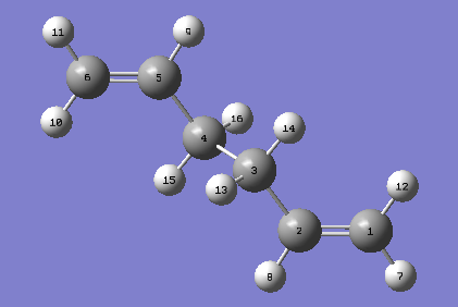
Optimisation of 1,5-hexadiene [anti1]

Molecule
Output Files	log / chk
Calculation Type	FOPT
Calculation Method	RHF
Basis Set	3-21G
Final Energy (au)	-231.69260235
Gradient (au)	0.00001824
Point Group	C2
Calculation Time (secs)	58

A molecule of 1,5-hexadiene with an 'anti' linkage for the central carbon atoms was created using GaussView 5.0. The molecule was then optimised using the Hartree Fock method and 3-21G basis set. The 3-21G basis set is a low level basis set, leading to short calculation times but a low accuracy. The output files for this optimisation, along with other details, can be found in the table to the left. The RMS gradient was found to be close to zero [0.00001824 au], indicating that the optimisation had been completed; however, to double-check this, the output file was examined in order to make sure that the forces and displacements had converged:

Item Value Threshold Converged? Maximum Force 0.000056 0.000450 YES RMS Force 0.000010 0.000300 YES Maximum Displacement 0.001388 0.001800 YES RMS Displacement 0.000459 0.001200 YES Predicted change in Energy=-2.090888D-08 Optimization completed. -- Stationary point found.

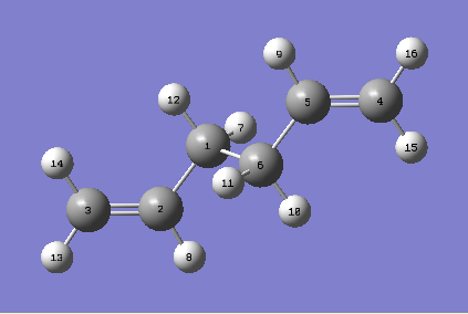
Optimisation of 1,5-hexadiene [gauche1]

In n-butane, the anti form is much more stable than the gauche form due to additional σ C-H / σ* C-H orbital interactions possible in this conformation. As 1,5-hexadiene is a similar-looking molecule, the same result might be expected for its anti and gauche forms; however, in previous studies, it has actually been found that there is a negligible energy difference between the anti and gauche forms. A possible explanation for this observation that has been proposed in literature is that there is an additional attractive interaction between the π electrons of the C=C bond and the vinyl protons in the gauche forms of 1,5-hexadiene that is not present in n-butane.

Molecule
Output Files	log / chk
Calculation Type	FOPT
Calculation Method	RHF
Basis Set	3-21G
Final Energy (au)	-231.68771617
Gradient (au)	0.00000542
Point Group	C1
Calculation Time (secs)	383

To test the above, a molecule of 1,5-hexadiene with a 'gauche' linkage for the central carbon atoms was created using GaussView 5.0. The molecule was then optimised using the Hartree Fock method and 3-21G basis set; this was the same method and basis set as the ones used above to allow comparison. As above, though the RMS gradient was found to be close to zero [0.00000542 au], indicating that the optimisation had been completed, the output file was checked in order to ensure that the forces and displacements had converged:

Item Value Threshold Converged? Maximum Force 0.000010 0.000450 YES RMS Force 0.000003 0.000300 YES Maximum Displacement 0.000215 0.001800 YES RMS Displacement 0.000058 0.001200 YES Predicted change in Energy=-4.666677D-09 Optimization completed. -- Stationary point found.

The difference in energy between the anti form of 1,5-hexadiene optimised above and the gauche form is 3.07 kcal/mol. Though this is a larger energy difference than expected, on closer inspection of the gauche conformer, it can be seen that due to the close proximity of the vinyl protons on C1 and C6 [3.13 Å], this is unlikely to be the lowest energy gauche conformer. However, the vinyl protons are not close enough to cause any significant steric repulsion and therefore, the energy of this gauche conformer is not much greater than that of the anti conformer.

Conformers of 1,5-hexadiene

There are, in fact, a total twelve rotational isomers of 1,5-hexadiene; however, as this includes two enantiomeric pairs, only the ten energetically different conformers have been listed below. All ten structures were optimised using the HF method at the 3-21G level of theory to allow comparison.

Conformer		Point Group	Energy (au)	Relative Energy (kcal/mol)		Conformer		Point Group	Energy (au)	Relative Energy (kcal/mol)
gauche 1 [log]		C2	-231.68771617	3.10		anti 1 [log]		C2	-231.69260235	0.04
gauche 2 [log]		C2	-231.69166702	0.62		anti 2 [log]		Ci	-231.69253528	0.08
gauche 3 [log]		C1	-231.69266114	0.00		anti 3 [log]		C2h	-231.68907066	2.25
gauche 4 [log]		C2	-231.69153035	0.71		anti 4 [log]		C1	-231.69097055	1.06
gauche 5 [log]		C1	-231.68961572	1.91
gauche 6 [log]		C1	-231.68916019	2.20

From the table above, it can be seen that though the energies of the conformers are similar, five of the conformers [gauche 1, gauche 5, gauche 6, anti 3, anti 4] have slightly higher energies than the rest. This is because their respective conformations are such that the vinyl protons are in close proximity, leading to unfavourable steric interactions. The lowest energy conformer of 1,5-hexadiene is gauche 3 in which these interactions are the least significant.

Optimisation of 1,5-hexadiene [anti2] Using a Higher Level Basis Set

Output Files	log
Calculation Type	FOPT
Calculation Method	RB3LYP
Basis Set	6-31G(d)
Final Energy (au)	-234.61170280
Gradient (au)	0.00001326
Dipole Moment (Debye)	0.0000
Point Group	Ci
Calculation Time (secs)	161.8

As the initial optimisation of the Ci anti2 conformer of 1,5-hexadiene was done using a low level basis set which only provides a rough approximation of the structure, the molecule was re-optimised using the higher level 6-31G(d) basis set.

Item Value Threshold Converged? Maximum Force 0.000015 0.000450 YES RMS Force 0.000006 0.000300 YES Maximum Displacement 0.000219 0.001800 YES RMS Displacement 0.000079 0.001200 YES Predicted change in Energy=-1.588835D-08 Optimization completed. -- Stationary point found.

The structure obtained from the optimisation at the 6-31G(d) level of theory appears to be virtually the same as the structure obtained at the 3-21G level; however, there are slight differences in the bond lengths and bond angles as seen in the table below:

		Bond Lengths (Å)				Bond Angles
			HF/3-21G	B3LYP/6-31G(d)			HF/3-21G	B3LYP/6-31G(d)
		C(1)-C(2)	1.32	1.33		C(1)-C(2)-C(3)	124.8°	125.3
		C(2)-C(3)	1.51	1.50		C(2)-C(3)-C(4)	111.3°	112.7
		C(3)-C(4)	1.55	1.55

Though the bond angles and distances of the structures obtained with the 3-21G and 6-31G(d) basis sets are almost identical, meaning that the lower level basis set is good at approximating the geometry of the lowest energy structure, the energies differ by 1832 kcal/mol. As this is a significant difference in energy, it can be concluded that in order to get reliable results from any further calculations, the structure should always be optimised using a sufficiently high level basis set beforehand.

Frequency Analysis of 1,5-hexadiene

A frequency analysis is carried out to ensure that the optimised structure is in its most stable ground state rather than in the transition state. This is done by calculating the second derivative of the potential energy surface and examining the frequencies obtained: if all the frequencies are real and positive then a minimum has been found, corresponding to the ground state, but if one of the frequencies is negative, a maximum has been found, corresponding to the transition state.

Output Files	log
Calculation Type	FREQ
Calculation Method	RB3LYP
Basis Set	6-31G(d)
Final Energy (au)	-234.61170280
Gradient (au)	0.00001300
Dipole Moment (Debye)	0.0000
Point Group	Ci
Calculation Time (secs)	188.6

A frequency analysis was carried out the optimised 1,5-hexadiene molecule to ensure that the minimum energy structure had been obtained. The calculation was done using the same method and basis set as the ones used in the optimisation as changing the basis set changes the accuracy of the calculation, resulting in different energies. Examination of the log file showed that there were no imaginary frequencies; this implied that the minimum energy structure had been found.

Low frequencies --- -18.6255 -11.7198 0.0003 0.0011 0.0012 1.8142 Low frequencies --- 72.7260 80.1435 120.0224

The energy of the molecule on the potential energy surface was found at 298.15 K and 0.00 K and have been tabulated below, along with the enthalpy and Gibbs Free energy. The energy at 298.15 K was obtained directly from the log file whilst the energy at 0.00 K was computed using the FreqChk utility.

	298.15 K	0.00 K
Sum of electronic and zero-point Energies (au)	-234.469212	-234.469212
Sum of electronic and thermal Energies (au)	-234.461856	-234.469212
Sum of electronic and thermal Enthalpies (au)	-234.460912	-234.469212
Sum of electronic and thermal Free Energies (au)	-234.500821	-234.469212

The 'sum of electronic and zero-point energies' is the zero-point-corrected electronic energy [E0 = Eelec + ZPE] whilst the 'sum of electronic and thermal energies' is the thermal-corrected energy that also includes the contributions from the translational, rotational and vibrational modes [E = E0 + Etrans + Erot + Evib]. Using the thermal-corrected energy, Gaussian also computes the predicted enthalpy [H = E + RT] and Gibbs Free Energies [G = H - TS] and these are the 'sum of electronic and thermal enthalpies' and 'sum of electronic and thermal Free Energies' in the table above.

If the energies at the two different temperatures are compared, it can be seen that the zero-point-corrected electronic energy does not change as the temperature is changed; this makes sense as the zero-point-corrected electronic energy is always calculated at 0.00 K. In addition to this, the thermal-corrected energy and zero-point-corrected energy at 0.00 K are exactly the same. This is because at absolute zero, no additional contributions from the translational, rotational and vibrational modes are expected.

OPTIMISING THE 'CHAIR' AND 'BOAT' TRANSITION STATES

During the optimisation process, Gaussian attempts to find the lowest energy structure at which the gradient of the potential energy surface is zero by solving the Schrodinger equation for the nuclear positions and electrons at different points along the potential energy surface. Though both the minimum [ground state] and maximum [transition state] of the potential energy surface have a first derivative equal to zero, their second derivatives are different: the curvature of the potential energy surface is positive at the minimum and negative at the maximum. Optimising transition states is more difficult than optimising to the ground state as the calculations will only converge to the transition state if the guess structure falls within the quadratic region of the true transition state - this region is normally much smaller than for the minimum ground state. The transition structures of the chair and boat have been optimised using several different methods and these have been discussed and compared in this section.

Optimisation of an Allyl Fragment

Structure
Output Files	log / chk
Calculation Type	FOPT
Calculation Method	UHF
Basis Set	3-21G
Final Energy (au)	-115.82304010
Gradient (au)	0.00003049
Point Group	C1
Calculation Time (secs)	9.0

Since the chair and boat transition structures both consist of two allyl fragments positioned 2.20 Å apart [but with different symmetries], an optimisation of an allyl fragment was first carried out using the Hartree-Fock method and 3-21G basis set. As discussed above, though the RMS gradient was found to be close to zero [0.00003049 au], indicating that the optimisation had completed successfully, the output file was checked in order to ensure that the forces and displacements had converged:

Item Value Threshold Converged? Maximum Force 0.000048 0.000450 YES RMS Force 0.000018 0.000300 YES Maximum Displacement 0.000141 0.001800 YES RMS Displacement 0.000070 0.001200 YES Predicted change in Energy=-1.277267D-08 Optimization completed. -- Stationary point found.

Optimisation of the Chair Transition State by Computing the Hessian

The Hessian, also known as the force constant matrix, gives the force constants of the harmonic vibrations of the molecule by computing the second derivatives of the energy with respect to the nuclear positions. This can be used to locate the transition state as at the transition state, there is one direction of downwards curvature [it is a first-order saddle point] and therefore, the transition state will have one negative Hessian eigenvalue and one imaginary frequency.

Structure
Output Files	log / chk
Calculation Type	FREQ
Calculation Method	RHF
Basis Set	3-21G
Final Energy (au)	-231.61932237
Gradient (au)	0.00002382
Point Group	C1
Calculation Time (secs)	10.0

First, the allyl fragment was duplicated and arranged in a 'chair'-like transition state, making sure that the distance between the terminal ends of the allyl fragments were approximately 2.20 Å apart. The transition state was then optimised using the Hartree Fock method and 3-21G basis set, using the command 'Optimisation to a TS (Berny)', choosing to calculate the force constants once and including the additional keywords Opt=NoEigen. These keywords were used to prevent the calculation from stopping if more than one imaginary frequency was obtained; this could have happened if the transition structure was not good enough and the critical point could not be found.

To ensure that the optimisation had completed successfully, the log file was examined to ensure that all the forces and displacements had converged:

Item Value Threshold Converged? Maximum Force 0.000069 0.000450 YES RMS Force 0.000011 0.000300 YES Maximum Displacement 0.000815 0.001800 YES RMS Displacement 0.000204 0.001200 YES Predicted change in Energy=-8.411719D-08 Optimization completed. -- Stationary point found.

At the transition state, there is only one direction of negative curvature so there should only be one imaginary frequency. Examination of the log file showed that there was an imaginary frequency at -818 cm-1, indicating that the transition structure had been located. If this vibration is animated, it can be seen that the vibration corresponds to the Cope rearrangement:

Low frequencies --- -817.9466 -2.3522 -0.0002 0.0002 0.0004 3.7204 Low frequencies --- 4.6153 209.4891 395.6909 ****** 1 imaginary frequencies (negative Signs) ******

Locating the transition state by computing the Hessian is a good method to use if the guess transition structure is reasonable. However, if the guess transition structure is far away from the true transition structure then the search may fail as the curvature may be too different.

Optimisation of the Chair Transition Structure by Freezing the Coordinates

Another method of locating the transition structure is by freezing the reaction coordinate and minimising the rest of the molecule. The reaction coordinate is then unfrozen and the optimisation is restarted. This can give a better transition structure and also save time as the whole Hessian may not need to be computed.

Structure
Output Files	log/chk
Calculation Type	FOPT
Calculation Method	RHF
Basis Set	3-21G
Final Energy (au)	-231.61478391
Gradient (au)	0.00352667
Point Group	C1
Calculation Time (secs)	29.0

First, the terminal carbons in the allyl fragments which form or break a bond during the rearrangment were frozen. This was done by changing 'Unidentified -> Bond' and 'Add -> Freeze Coordinate' in the Redundant Coordinate Editor. The transition structure was then optimised, making sure that the keywords Opt=ModRedundant were present, and the resulting log file was checked to ensure that all the forces and displacements had converged:

Item Value Threshold Converged? Maximum Force 0.000031 0.000450 YES RMS Force 0.000008 0.000300 YES Maximum Displacement 0.000757 0.001800 YES RMS Displacement 0.000179 0.001200 YES Predicted change in Energy=-9.585268D-08 Optimization completed. -- Stationary point found.

The optimised structure was similar to the transition state optimised by calculating the Hessian except that the bond forming/breaking distances were fixed. To optimise these distances, the frozen bonds were selected and the parameters 'Unidentified' and 'Add' were changed to 'Bond' and 'Derivative' respectively using the Redundant Coordinate Editor.

Structure
Output Files	log/chk
Calculation Type	FREQ
Calculation Method	RHF
Basis Set	3-21G
Final Energy (au)	-231.61932225
Gradient (au)	0.00002477
Point Group	C1
Calculation Time (secs)	9.0

A second transition state optimisation was carried out on the structure in a similar way as above but in this case, the force constants were not calculated. Instead, a normal guess Hessian was used that was modified to include information about the two coordinates that the differentiation was taking place along. To ensure that the optimisation had completed, the log file was examined to ensure that all the forces and displacements had converged:

Item Value Threshold Converged? Maximum Force 0.000082 0.000450 YES RMS Force 0.000024 0.000300 YES Maximum Displacement 0.001397 0.001800 YES RMS Displacement 0.000384 0.001200 YES Predicted change in Energy=-2.031608D-07 Optimization completed. -- Stationary point found.

Examination of the log file showed that there was one imaginary frequency at 818 cm-1 as expected, implying that the structure found was the transition state. By animating this vibration, it can be seen that this corresponds to the Cope rearrangement:

Low frequencies --- -817.8611 -1.9884 0.0003 0.0005 0.0007 5.2915 Low frequencies --- 7.9943 209.6078 396.0162 ****** 1 imaginary frequencies (negative Signs) ******

Comparison of the Chair Transition Structures Obtained via Different Methods

The bond forming/breaking distances of the chair transition structures obtained via the two methods carried out have been tabulated below:

	Hessian Method	Frozen Coordinate Method
Bond Forming/Breaking Distance (Å)	2.02092	2.02048
	2.02105	2.02049

Alhough there is a slight variation in the bond forming/breaking distances of the two chair transition structures, computed bond distances are generally only accurate to 0.01 Å. Both chair transition structures have bond breaking/forming distances of 2.02 Å to two decimal places and can therefore be considered almost identical.

Optimising the Boat Transition State via the QST2 Method

In the QST2 [quadratic synchronous transit] method, both the reactants and products are specified. The calculation then uses these two points on the potential energy surface and linearly interpolates a line between them in order to make an approximation of the reaction pathway. The maximum point is then minimised perpendicular to the direction of the pathway and a new quadratic pathway is interpolated using the minimised maximum, the reactant and the product. The transition structure obtained from the QST2 method is the maximum point of the quadratic pathway.

For the QST2 method to work successfully, the numbering of the reactants and products must be identical. The optimised Ci anti2 reactant molecule from above was therefore duplicated, arranged and renumbered {reactant, product}. An optimisation and frequency calculation was attempted using the QST2 method but the calculation failed. When the checkpoint file was opened, the following structure was obtained:

The obtained structure appeared to resemble the chair transition structure more than the boat transition structure. This was thought to be because the reactant and product structures used were too far away from the structure of the real boat transition state and therefore, when the linear interpolation was carried out in order to estimate the approximate reaction pathway, the calculation just translated one of the allyl fragments and did not consider rotating the central bonds. In order to obtain the boat transition structure by the QST2 method, it is therefore necessary to change the geometry of the starting structures and products so that they resemble that of the boat transition state. Keeping this in mind, the central C-C-C-C dihedral angles were set to 0o and the inside C-C-C angles were set to 100o. This gave the following geometries for the reactant and product:

Output Files	log/chk
Calculation Type	FREQ
Calculation Method	RHF
Basis Set	3-21G
Final Energy (au)	-231.60280216
Gradient (au)	0.00005453
Point Group	Cs
Calculation Time (secs)	8.0

A QST2 calculation was set up using the same method as above and this time, the job successfully converged to the boat transition structure.

Item Value Threshold Converged? Maximum Force 0.000054 0.000450 YES RMS Force 0.000023 0.000300 YES Maximum Displacement 0.000823 0.001800 YES RMS Displacement 0.000227 0.001200 YES Predicted change in Energy=-1.496032D-07 Optimization completed. -- Stationary point found.

Examination of the log file showed that there was one imaginary frequency at -840 cm-1, implying that the transition state had been found. The motion of this vibration is shown below:

Low frequencies --- -839.8775 -7.8696 -3.5974 -0.0002 0.0006 0.0009 Low frequencies --- 2.3147 154.9331 381.9746 ****** 1 imaginary frequencies (negative Signs) ******

Optimising the Boat Transition State via the QST3 Method

The QST3 method allows a guess of the geometry of the transition state to be inputted, generally leading to more reliable results.

Output Files	log/chk
Calculation Type	FREQ
Calculation Method	RHF
Basis Set	3-21G
Final Energy (au)	-231.60280168
Gradient (au)	0.00004906
Point Group	C1
Calculation Time (secs)	8.0

A QST3 calculation was carried out on the original 1,5-hexadiene reactant/product molecules [with all angles unchanged] and this 'guess' transition state.

Item Value Threshold Converged? Maximum Force 0.000117 0.000450 YES RMS Force 0.000024 0.000300 YES Maximum Displacement 0.001276 0.001800 YES RMS Displacement 0.000379 0.001200 YES Predicted change in Energy=-1.896673D-07 Optimization completed. -- Stationary point found.

Examination of the log file showed that there was one imaginary frequency at -841 cm-1, implying that the transition state had been found. The motion of this vibration is shown below:

Low frequencies --- -840.7640 -7.6871 -5.7518 -3.4177 -0.0001 0.0003 Low frequencies --- 0.0009 154.9884 382.7834 ****** 1 imaginary frequencies (negative Signs) ******

If the structure obtained from the QST3 method is compared to that obtained from the QST2 method, it can be seen that the two transition states are very similiar.

Intrinsic Reaction Coordinate

Starting from the transition state, the IRC method follows the path of steepest descent from this point on the potential energy surface to its local minimum. The path can be followed in the forward and backwards direction, leading to two minima, one corresponding to the reactants and one corresponding to the products.

IRC Method [Chair Transition Structure]

Output Files	log
Calculation Type	IRC
Final Energy (au)	-231.69157875
Gradient (au)	0.00015223
Point Group	C1
Calculation Time (secs)	274

The intrinsic reaction coordinate [IRC] method was carried out on the optimised chair transition structure. This was done by selecting IRC under the Job Type, computing the reaction in the forward direction [as the reaction coordinate in this case is symmetrical], calculating the force constants at every step and using a total of 50 points. Though the last point on the IRC showed a structure that closely resembled conformer gauche 2, its energy was slightly higher than expected, indicating that it had not yet reached the minimum geometry. This structure was therefore taken and used to run a normal minimisation calculation as shown below:

Optimised Structure
Output Files	log
Calculation Type	FOPT
Calculation Method	RHF
Basis Set	3-21G
Final Energy (au)	-231.69166702
Gradient (au)	0.00000030
Point Group	C2
Calculation Time (secs)	10.0

As for all the optimisations carried out, although the RMS gradient was close to zero [0.00000030 au], the log file was checked to ensure that all the forces and displacements had converged.

Item Value Threshold Converged? Maximum Force 0.000001 0.000450 YES RMS Force 0.000000 0.000300 YES Maximum Displacement 0.000350 0.001800 YES RMS Displacement 0.000117 0.001200 YES Predicted change in Energy=-1.586291D-10 Optimization completed. -- Stationary point found.

As stated in the Conformers of 1,5-hexadiene section, the energy of the optimised conformer gauche 2 at the HF/3-21G level of theory is -231.69166702 au. As this is identical to the energy obtained in this optimisation, it can be concluded that the minimum geometry has been obtained.

IRC Method [Boat Transition Structure]

Output Files	log
Calculation Type	IRC
Final Energy (au)	-231.69261285
Gradient (au)	0.00013415
Point Group	C1
Calculation Time (secs)	1464.4

The intrinsic reaction coordinate [IRC] method was also carried out on the optimised boat transition structure. This was done by selecting IRC under the Job Type, computing the reaction in the forward direction [as the reaction coordinate in this case is symmetrical], calculating the force constants at every step and using a total of 100 points. Though the last point on the IRC showed a structure that closely resembled conformer gauche 3, its energy was slightly higher than expected, indicating that it had not yet reached the minimum geometry. This structure was therefore taken and used to run a normal minimisation calculation as shown below:

Optimised Structure
Output Files	log
Calculation Type	FOPT
Calculation Method	RHF
Basis Set	3-21G
Final Energy (au)	-231.69266121
Gradient (au)	0.00001131
Point Group	C1
Calculation Time (secs)	36.9

As for all the optimisations carried out, although the RMS gradient was close to zero [0.00001131 au], the log file was checked to ensure that all the forces and displacements had converged.

Item Value Threshold Converged? Maximum Force 0.000030 0.000450 YES RMS Force 0.000008 0.000300 YES Maximum Displacement 0.001298 0.001800 YES RMS Displacement 0.000265 0.001200 YES Predicted change in Energy=-1.775442D-08 Optimization completed. -- Stationary point found.

As stated in the Conformers of 1,5-hexadiene section, the energy of the optimised conformer gauche 3 at the HF/3-21G level of theory is -231.69266114 au. As this is almost the same as the energy obtained in this optimisation, it was concluded that the minimum geometry is the gauche 3 conformer.

ACTIVATION ENERGIES FOR THE REACTION

To calculate the activation energies for the reaction via the chair and boat transition structures, both transition structures were reoptimised using the higher level B3LYP/6-31G(d) level of theory. As seen from the optimisation of 1,5-hexadiene to the 6-31G(d) level of theory, the geometries obtained from using the 3-21G and 6-31G(d) basis sets are virtually identical but their energies are significantly different. The same observation is expected for the reoptimisation of the chair and boat transition states:

Chair			Boat
Output File	log		Output File	log
Calculation Type	FREQ		Calculation Type	FREQ
Calculation Method	RB3LYP		Calculation Method	RB3LYP
Basis Set	6-31G(d)		Basis Set	6-31G(d)
Final Energy (au)	-234.55698303		Final Energy (au)	-234.54309307
Gradient (au)	0.00001207		Gradient (au)	0.00000486
Dipole Moment (Debye)	0.00		Dipole Moment (Debye)	0.06
Point Group	C1		Point Group	Cs
Calculation Time (secs)	158		Calculation Time (secs)	87

The computed bond lengths and angles for the chair and boat transition structures have been tabulated below. As the transition structures are symmetrical, only the key distances have been recorded.

Chair Transition Structure

		Bond Lengths (Å)
			HF/3-21G	B3LYP/6-31G(d)
		C(1)-C(2)	1.39	1.41
		C(3)-C(6)	2.02	1.97
		Bond Angles (Å)
			HF/3-21G	B3LYP/6-31G(d)
		C(1)-C(2)-C(3)	120.1°	120.0°

Boat Transition Structure

		Bond Lengths (Å)
			HF/3-21G	B3LYP/6-31G(d)
		C(1)-C(2)	1.38	1.39
		C(3)-C(6)	2.14	2.21
		Bond Angles (Å)
			HF/3-21G	B3LYP/6-31G(d)
		C(1)-C(2)-C(3)	121.6°	122.3°

As expected, changing the basis set from 3-21G to 6-31G(d) did not alter the geometry of the transition structures by much. However, the electronic energies were found to be significantly different [as seen in the table below], meaning that though the 3-21G basis set can be used to obtain a rough approximation of the optimised structure, the structures should always be reoptimised at the higher level 6-31G(d) basis set. As calculations at the 6-31G(d) level can be time-consuming, it is often a good idea to optimise at a lower level basis set first and then reoptimise.

In literature, the boat conformer has been found to be less stable than the chair conformer by approximately 5-6 kcal/mol. This is due to two reasons:

Firstly, as seen from the diagram to the left, the boat conformation is eclipsed, leading to a higher degree of torsional strain, destabilising the molecule. In addition to this, there are additional Van der Waals repulsions between the 'flagpole' hydrogens which are in close proximity to each other. As both these effects are beginning to become significant in the transition state, it is expected that the boat transition state will be of higher energy than the chair transition state. In the calculations above, the energy of the boat transition state was found to be -234.54309307 au whilst the energy of the chair transition state was found to be -234.55698303 au; the energy of the boat was therefore found to be higher than the energy of the chair, agreeing with literature findings.

Activation Energies

	HF/321-G				B3LYP/6-31G(d)
	Electronic Energy	Sum of Electronic and Zero-Point Energies at 0 K	Sum of Electronic and Thermal Energies at 298.15 K		Electronic Energy	Sum of Electronic and Zero-Point Energies at 0 K	Sum of Electronic and Thermal Energies at 298.15 K
Chair TS	-231.619322	-231.466703	-231.461342		-234.556983	-234.414929	-234.409009
Boat TS	-231.602802	-231.450925	-231.445295		-234.543093	-234.402342	-234.396008
anti2	-231.692535	-231.539539	-231.532565		-231.532565	-234.469212	-234.461856
		Activation Energy at 0 K	Activation Energy at 298.15 K		Activation Energy at 0 K	Activation Energy at 298.15 K
ΔE (Chair)/kcal mol-1		45.71	44.69		34.06	33.16
ΔE (Boat)/kcal mol-1		55.61	54.76		41.96	41.32

As the electronic energy for the boat transition state is higher than that for the chair transition state, the activation energy of the reaction via the boat transition state should be higher than the reaction via the chair transition state - this can be seen from the table above. The experimentally-determined activation energies are 33.5 ± 0.5 kcal/mol via the chair transition structure and 44.7 ± 2.0 kcal/mol via the boat transition structure at 0 K. Clearly, the activation energies obtained using the 6-31G(d) basis set agree better with the experimental values than those obtained at the 3-21G level of theory; this makes sense as the 6-31G(d) basis set is a higher level basis set and is therefore expected to give more accurate results. Also, though the values computed at the 6-31G(d) level of theory are not exactly the same as the experimental values, they are very close: for the activation energy of the chair transition state, there is a percentage error of approximately 2% whilst for the activation energy of the boat transition state, the percentage error is approximately 6%.

PART 2 : THE DIELS-ALDER CYCLOADDITION OF cis-BUTADIENE AND ETHYLENE

The Diels-Alder reaction between cis-butadiene and ethylene is a pericyclic reaction [or, more specifically, a [π4s + π2s] cycloaddition] in which the π orbitals of cis-butadiene interact with the π orbitals of ethylene to form two new σ bonds. The total electron count is 6, which fits the 4n+2 rule, and so, the thermal reaction should proceed suprafacially via a Hückel aromatic transition state.

In general, the HOMO/LUMO of the diene interacts with the HOMO/LUMO of the dienophile to form two new bonding and antibonding molecular orbitals. This can only occur between molecular orbitals of the same symmetry as sufficient overlap of electron density is required. In this section, the molecular orbitals of the reactants and transition state have been computed in order to investigate this statement further.

Optimisation of cis-butadiene

Molecule
Output Files	log / chk
Calculation Type	FOPT
Calculation Method	RAM1
Basis Set	ZDO
Final Energy (au)	0.04879719
Gradient (au)	0.00001745
Point Group	C1
Calculation Time (secs)	8

To start, a molecule of cis-butadiene was created in Gaussview. An optimisation calculation was then carried out using the semi-empirical AM1 molecular orbtital method. The RMS gradient was found to be close to zero [0.00001745 au], indicating that the optimisation had been completed; however, to double-check this, the output file was examined in order to make sure that the forces and displacements had converged:

Item Value Threshold Converged? Maximum Force 0.000030 0.000450 YES RMS Force 0.000011 0.000300 YES Maximum Displacement 0.000373 0.001800 YES RMS Displacement 0.000162 0.001200 YES Predicted change in Energy=-9.691106D-09 Optimization completed. -- Stationary point found.

The HOMO and LUMO of cis-butadiene were visualised using the checkpoint file, giving the following:

HOMO		LUMO
ANTISYMMETRIC		SYMMETRIC

If the symmetry of the HOMO and LUMO are determined with respect to the plane of symmetry between the two central carbon atoms, the HOMO is found to be antisymmetric whilst the LUMO is found to be symmetric.

Locating the Transition State via the QST3 Method

Output Files	log/fchk
Calculation Type	FREQ
Calculation Method	RAM1
Basis Set	ZDO
Final Energy (au)	0.11165464
Gradient (au)	0.00000078
Point Group	C1
Calculation Time (secs)	6.9

To locate the transition structure, a QST3 calculation was carried out using the optimised reactant and product structures and this 'guess' transition state.

Item Value Threshold Converged? Maximum Force 0.000002 0.000450 YES RMS Force 0.000000 0.000300 YES Maximum Displacement 0.000080 0.001800 YES RMS Displacement 0.000021 0.001200 YES Predicted change in Energy=-8.932061D-11 Optimization completed. -- Stationary point found.

Examination of the log file showed that there was one imaginary frequency at -956 cm-1, implying that the transition state had been found:

Low frequencies --- -956.2246 -1.6085 -0.0693 -0.0032 0.0216 2.1087 Low frequencies --- 2.3554 147.2482 246.6363 ****** 1 imaginary frequencies (negative Signs) ******

From the animation above, it can be seen that the vibration corresponding to the imaginary frequency is synchronous and does not break the symmetry of the molecule. In contrast to this, the vibration corresponding to the lowest positive frequency is asynchronous and breaks symmetry. Remembering that at the transition state, there is only one direction of downwards curvature and therefore just one imaginary frequency, the fact that the frequency of the asynchronous vibration is real implies that motion along this direction is uphill in energy. In other words, the only motion that leads to a decrease in energy is the motion corresponding to the imaginary frequency. As this motion happens to be synchronous, the Diels-Alder cycloaddition must involve the concerted formation of two sigma bonds, conserving symmetry.

The Geometry of the Transition State

The bond length of a typical C(sp2)=C(sp2) double bond is 1.31-1.34 Å. In the reactant molecules, there are C=C double bonds between C(1)-C(2), C(3)-C(4) and C(5)-C(6). From the annotated diagram to the left, it can be seen that the bond between these carbon atoms are longer, indicating that there has been a reduction in bond order [the double bonds are becoming more like single bonds] as expected from the Diels-Alder reaction. In addition to this, it can be seen that the bond between C(2)-C(3) is shorter than expected, given that a typical conjugated C(sp2)-C(sp2) bond has a bond length of 1.45-1.46 Å. This shortening of the bond indicates an increase in bond order; in other words, the single bond is moving towards becoming a double bond. Again, this change is as expected from the Diels-Alder reaction.

The Van der Waals radius of a carbon atom is 1.70 Å. As the C(1)-C(5) interfragment distance of 2.12 Å is much shorter than the sum of the Van der Waals radii [3.40 Å] but greater than that of a typical C(sp3)-C(sp3) single bond [1.53-1.55 Å], it can be concluded that a bond is beginning to form. In addition to this, it should be noted that the two interfragment distances [C(1)-C(5) and C(4)-C(6)] are identical, supporting the idea that the two sigma bonds form in a concerted fashion.

Molecular Orbitals

In a cycloaddition, the HOMO of one fragment interacts with the LUMO of the other fragment in order to form two new sigma bonds. For this to happen, the orbitals must have the same symmetry. If the frontier molecular orbitals of ethylene and butadiene are considered:

The HOMO and LUMO of butadiene and ethylene can be labelled symmetric or antisymmetric with respect to the plane of symmetry between the central two carbons as shown above. As only molecular orbitals of the same symmetry can interact, there are two possible HOMO/LUMO combinations, one involving the symmetric HOMO of ethylene and the symmetric LUMO of butadiene, and the other involving the antisymmetric HOMO of butadiene and the antisymmetric LUMO of ethylene. This leads to the formation of four molecular orbitals - two bonding and two antibonding - as shown below:

		HOMO		LUMO
-0.32499 au		-0.32394 au		0.02315 au		0.03378 au
SYMMETRIC		ANTISYMMETRIC		SYMMETRIC		ANTISYMMETRIC

Generally, Diels-Alder reactions occur between electron-rich dienes and electron-deficient dienophiles. Increasing the electron-deficiency of the dienophile [for example, by adding an electron-withdrawing substituent] lowers the HOMO/LUMO energies of the dienophile and makes the overlap between the HOMO(diene)/LUMO(dienophile) more favourable than the overlap between the HOMO(dienophile)/LUMO(diene). In this case, the dienophile is a simple ethylene molecule, meaning that its HOMO and LUMO are relatively high. The HOMO(diene)/LUMO(dienophile) energy gap is therefore expected to be similar to the HOMO(dienophile)/LUMO(diene) energy gap and both combinations are equally likely. From examination of the molecular orbitals above, it can be seen that as predicted, the energies of the two bonding orbitals are similar and the energies of the two antibonding orbitals are similar. The HOMO was found to be antisymmetric with respect to the plane of symmetry indicated and as shown in the diagram above, it is made up of the antisymmetric HOMO of butadiene and the antisymmetric LUMO of ethylene. This is allowed as the symmetry of both fragments is such that there is a bonding interaction where the two new sigma bonds are going to form.

PART 3: THE REGIOSELECTIVITY OF THE DIELS-ALDER REACTION

Unlike the reaction between cis-butadiene and ethylene discussed above, the issue of regioselectivity must be considered in the reaction of cyclohexa-1,3-diene and maleic anhydride. There are two possible products - the exo adduct and the endo adduct - depending on the orientation of the reactants relative to each other:

Though the exo adduct is more stable and is therefore the preferred product in reversible Diels-Alder reactions, it is the less stable endo product that dominates in irreversible Diels-Alder reactions, meaning that it must be the kinetic product. This means that the endo transition state should be more stable than the exo transition state, leading to the endo product being formed at a faster rate. In this section, the reasons why the endo transition state is more stable than the exo transition state are investigated.

Optimisation of the Reactants and the Products

To locate the transition structures of the exo and endo adducts via the QST3 method, the reactants and products were first optimised:

Cyclohexadiene			Maleic Anhydride
Structure			Structure
Output File	log		Output File	log
Calculation Type	FOPT		Calculation Type	FOPT
Method	RAM1		Method	RAM1
Basis Set	ZDO		Basis Set	ZDO
Final Energy (au)	0.02771129		Final Energy (au)	-0.12182423
Gradient (au)	0.00000562		Gradient (au)	0.00004090
Point Group	C2		Point Group	C1
Calculation Time (secs)	32.9		Calculation Time (secs)	25.9

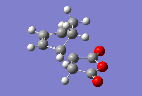
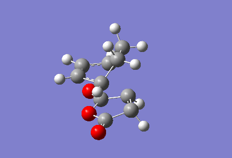
Exo Adduct			Endo Adduct
Structure			Structure
Output File	log		Output File	log
Calculation Type	FOPT		Calculation Type	FOPT
Method	RAM1		Method	RAM1
Basis Set	ZDO		Basis Set	ZDO
Final Energy (au)	-0.15990940		Final Energy (au)	-0.16017080
Gradient (au)	0.00000901		Gradient (au)	0.00002110
Point Group	C1		Point Group	C1
Calculation Time (secs)	64.6		Calculation Time (secs)	85.7

Finding the Exo Transition State

Output Files	log
Calculation Type	FREQ
Calculation Method	RAM1
Basis Set	ZDO
Final Energy (au)	-0.05041985
Gradient (au)	0.00000112
Point Group	C1
Calculation Time (secs)	8.3

To locate the transition structure, a QST3 calculation was carried out using the optimised reactant and product structures and this 'guess' transition state.

Item Value Threshold Converged? Maximum Force 0.000002 0.000450 YES RMS Force 0.000000 0.000300 YES Maximum Displacement 0.000106 0.001800 YES RMS Displacement 0.000030 0.001200 YES Predicted change in Energy=-9.560838D-11 Optimization completed. -- Stationary point found.

Examination of the log file showed that there was one imaginary frequency at -812 cm-1, implying that a transition state had been found. The transition structure and the motion of the imaginary vibration are shown below:

Low frequencies --- -812.2185 -1.4150 -1.3320 -0.0047 0.2200 1.0448 Low frequencies --- 2.0991 60.8548 123.8691 ****** 1 imaginary frequencies (negative Signs) ******

The vibration corresponding to the imaginary frequency is synchronous; this implies that the two new C-C sigma bonds are forming in a concerted fashion. As it is an imaginary frequency, motion along this degree of freedom must be downhill, leading to a decrease in energy.

Finding the Endo Transition State

Output Files	log
Calculation Type	FREQ
Calculation Method	RAM1
Basis Set	ZDO
Final Energy (au)	-0.05150480
Gradient (au)	0.00000305
Point Group	C1
Calculation Time (secs)	8.4

To locate the transition structure, a QST3 calculation was carried out using the optimised reactant and product structures and this 'guess' transition state.

Item Value Threshold Converged? Maximum Force 0.000007 0.000450 YES RMS Force 0.000001 0.000300 YES Maximum Displacement 0.000721 0.001800 YES RMS Displacement 0.000149 0.001200 YES Predicted change in Energy=-6.346012D-09 Optimization completed. -- Stationary point found.

Examination of the log file showed that there was one imaginary frequency at -806 cm-1, implying that a transition state had been found. The transition structure and the motion of the imaginary vibration are shown below:

Low frequencies --- -806.4327 -1.7695 -1.5904 -0.4510 -0.0104 0.4688 Low frequencies --- 1.3229 62.4178 111.7374 ****** 1 imaginary frequencies (negative Signs) ******

As seen above, the vibration corresponding to the imaginary frequency is synchronous, implying that symmetry is conserved in the Diels-Alder reaction. As the frequency is imaginary, this motion must lead to a decrease in energy.

The Geometry of the Exo and Endo Transition States

The Exo Transition State

The geometry of the exo transition state can be found in the diagram to the left where the white arrows represent bond distances and the blue arrows represent through-space distances. The bond length of a typical C(sp2)=C(sp2) double bond is 1.31-1.34 Å whilst the bond length of a typical C(sp2)-C(sp2) bond is approximately 1.53-1.55 Å. The bond lengths marked 1.39 Å and 1.41 Å were both C(sp2)=C(sp2)-type double bonds in the reactant molecules; both these bond lengths are now longer than would be expected for a typical C=C double bond, indicating that they are becoming more like single bonds. In contrast to this, the bond length marked 1.40 Å is where a conjugated C(sp2)-C(sp2) bond used to be; this type of bond would be expected to have a bond length of 1.45-1.46 Å so the fact that the bond length is now shorter than this must mean that the bond is gaining double bond character as expected.

The Van der Waals radius of the carbon atom is 1.70 Å. As the partly formed σ C-C bond length is much shorter than the sum of the Van der Waals radii [3.40 Å] but greater than that of a typical C(sp3)-C(sp3) single bond [1.53-1.55 Å], it can be concluded that a bond is beginning to form. The partly formed σ C-C bond length is the same on both sides, indicating that the two sigma bonds are forming simultaneously.

The Endo Transition State

The geometry of the endo transition state can be found in the diagram on the left. All the C-C bond distances marked with white arrows, along with the bond distance of the partly formed σ bond, are the same as in the exo form and can be rationalised in the same way. The key difference between the geometries of the exo and endo transition states is the orientation of the maleic anhydride relative to the cyclohexadiene. The C-C through space distance between the -(C=O)-O-(C=O)- fragment of the maleic anhydride and the 'opposite' carbons on the cyclohexadiene is 2.95 Å in the exo form and 2.89 Å in the endo form. Though this might suggest that there is more steric repulsion in the endo transition state, the close proximity of the two hydrogens on the exo transition state and the carbonyl carbons of the maleic anhydride [2.42 Å] means that the exo transition state is most likely more strained. This supports the fact that the energy of the endo transition state was found to be -0.05150480 au, making it more stable than the exo transition state of energy -0.05041985 au. The endo adduct is therefore formed faster and is the kinetic product.

Endo vs Exo Selectivity

In literature, the most widely accepted explanation for why the endo transition state is more stable than the exo transition state in Diels-Alder reactions is that there are additional 'secondary orbital overlap' interactions present in the endo form. However, there is actually very little experimental evidence supporting their existence, a fact that will be discussed in more detail in this section.

The 'Secondary Orbital Effect'

To understand the premise behind the secondary orbital effect, the molecular orbitals of the system should be visualised. Looking first at the HOMO and LUMO of the reactants, the following is obtained:

CYCLOHEXADIENE				MALEIC ANHYDRIDE
HOMO		LUMO		HOMO		LUMO
-0.32194 au		0.01680 au		-0.44186 au		-0.05949 au
ANTISYMMETRIC		SYMMETRIC		SYMMETRIC		ANTISYMMETRIC

Due to the electronegativity of oxygen and the electron-withdrawing carbonyl groups, the maleic anhydride dienophile is electron poor. This causes its LUMO/HOMO to be lower than that of a simple alkene, meaning that though there are two possible HOMO/LUMO combinations of the same symmetry [HOMO(diene)/LUMO(dienophile) and HOMO(dienophile)/LUMO(diene)], one is more favoured than the other. This can be seen more clearly if the frontier orbital diagram is constructed [ignoring the π orbitals of the carbonyl groups for now]:

The effect of lowering the HOMO/LUMOs of maleic anhydride is that the energy gap between the asymmetric HOMO of cyclohexadiene and the asymmetric LUMO of maleic anhydride is much smaller than the energy gap of the symmetric HOMO/LUMO combination. This means that during the Diels-Alder process, the electrons will be donated from the HOMO of the electron-rich diene into the LUMO of the electron-poor dienophile - this is normal electron demand. However, due to the additional substituents on the dienophile, unlike the reaction between cis-butadiene and ethylene discussed above, there are two possible orientations of the reactants that can occur, forming the exo and endo products respectively. If the HOMO of the exo and endo transition states are examined:

EXO HOMO		ENDO HOMO
ANTISYMMETRIC		ANTISYMMETRIC

Both HOMOs are antisymmetric as expected and are formed from the interaction of the antisymmetric LUMO of cyclohexadiene and the antisymmetric HOMO of maleic anhydride. To explain why the endo transition state is more stable than the exo transition state, it has been proposed that there are additional stabilising 'secondary orbital interactions' between the π orbitals of the carbonyl groups on maleic anhydride and the back π orbitals of the cyclohexadiene in the endo transition state. This has been illustrated below, where the black lines represent primary interactions and the red lines represent secondary interactions:

However, as mentioned at the beginning of this section, there is little clear experimental evidence to support the existence of secondary orbital effects and even if they do exist, the magnitude of these second-order interactions would be expected to be small. Alternative explanations that have been proposed in literature to explain the endo vs exo selectivity of Diels-Alder reactions include solvent effects, steric interactions, hydrogen bonds and electrostatic forces.

As discussed above, the exo transition state may be expected to be more sterically hindered than the endo transition state due to the close proximity of the two hydrogens on cyclohexadiene and the carbonyl carbons on maleic anhydride [2.42 Å]. However, their close proximity may also lead to the presence of repulsive electrostatic interactions taking place here; due to the high electronegativity of oxygen, the carbonyl carbons on maleic anhydride can be considered to be slightly positively charged and therefore, these carbons may be repelling the hydrogens, leading to a higher energy transition state. As this sort of interaction is thought to be present in the endo transition structure of isoprene and maleic anhydride where the distance between the hydrogen atoms and the carbonyl carbons are 2.60 Å, it is not hard to imagine that the same interaction could occur here as the through-space distance is shorter. However, further research is required to confirm whether this is indeed the case.

Solvent Effects

The choice of solvent used can also have an effect on the exo versus endo selectivity, as well as the rate of reaction. For example, the endo selectivity and rate of reaction has been found to increase when the reactions are carried out in water compared to when the reactions are carried out with no solvent or in hydrocarbon solvents. If the endo and exo transition structures are computed using the QST3 method and a water solvation model, the following is obtained:

Exo Transition State			Endo Transition State
Output File	log		Output File	log
Calculation Type	FREQ		Calculation Type	FREQ
Calculation Method	RAM1		Calculation Method	RAM1
Basis Set	ZDO		Basis Set	ZDO
Final Energy (au)	-0.06253334		Final Energy (au)	-0.06477763
Gradient (au)	0.00000086		Gradient (au)	0.00000223
Point Group	C1		Point Group	C1
Calculation Time (secs)	123.8		Calculation Time (secs)	125.4

If these energies are compared with the energies of endo and exo transition states computed with no solvent above,

No Solvent			Water Solvent
Exo	-0.05041985 au		Exo	-0.06253334 au
Endo	-0.05150480 au		Endo	-0.06477763 au

Two key observations can be made from the table above: firstly, the energies of both transition states obtained using a water solvation model are lower than the energies obtained without. Secondly, without solvent, the endo transition state is more stable than the exo transition state by 0.68 kcal/mol whilst with water as a solvent, the endo transition state is more stable by 1.41 kcal/mol. This means that the reaction between maleic anhydride and cyclohexadiene in water would be expected to occur faster and with higher endo selectivity, supporting experimental findings. The reason this occurs is because both maleic anhydride and cyclohexadiene are insoluble in water and form oily droplets, leading to them being placed in closer proximity to each other than they would be normally.

REFERENCES

- ↑ 1.0 1.1 1.2 1.3 O. Wiest, K. A. Black, K. N. Houk, "Density Functional Theory Isotope Effects and Activation Energies for the Cope and Claisen Rearrangements", J. Am. Chem. Soc., 1994, 116 (22), 10336-10337.DOI:10.1021/ja00101a078
- ↑ H. Rzepa, "Conformations of Saturated, Straight-Chain Hydrocarbons: σ-σ Conjugation", Conformational Analysis, 2nd Year
- ↑ B. G. Rocque, J. M. Gonzales, H. F. Schaefer, "An analysis of the conformers of 1,5-hexadiene", Molecular Physics: An International Journal at the Interface between Chemistry and Physics, 2002, 100 (4), 441-446.DOI:10.1080/00268970110081412
- ↑ 4.0 4.1 B. W. Gung, Z. Zhu, R. A. Fouch, "Conformational Study of 1,5-hexadiene and 1,5-Diene-3,4-diols", J. Am. Chem. Soc., 1995, 117 (6), 1783-1788.DOI:10.1021/ja00111a016
- ↑ "G09 Keywords: G1-G4", Gaussian 09 User's Reference
- ↑ 6.0 6.1 6.2 6.3 6.4 6.5 H. P. Hratchian, H. B. Schlegel, Finding minima, transition states, and following reaction pathways on ab initio potential energy surfaces, "Theory and Application of Computational Chemistry: The First Forty Years", Chapter 10, 2005, Elsevier B. V.
- ↑ P. Hunt, "Comments on accuracy, energies and symmetry", Computational Chemistry Labs, 3rd Year
- ↑ "G09 Keyword: IRC", Gaussian 09 User's Reference
- ↑ 9.0 9.1 9.2 9.3 9.4 E. V. Anslyn, D. A. Dougherty, "Modern Physical Organic Chemistry", 2006, University Science Books
- ↑ 10.0 10.1 10.2 10.3 10.4 10.5 10.6 J. Clayden, N. Greeves, S. Warren, P. Wothers, "Organic Chemistry", 2009, Oxford University Press
- ↑ 11.0 11.1 11.2 11.3 11.4 J. I. Garcia, J. A. Mayoral, L. Salvatella, "Do Secondary Orbital Interactions Really Exist?", Acc. Chem. Res., 2000, 33 (10), 658-664.DOI:10.1021/ar0000152