Rep:Mod:otr12CMP
Third year CMP compulsory experiment
TASK: Show that the lowest possible energy for the Ising model is , where is the number of dimensions and is the total number of spins. What is the multiplicity of this state? Calculate its entropy.
Equation 1: The total interaction energy for the Ising Model
To compute the lowest possible energy, one needs to consider the total interaction energy given by equation 1. The summations over all spins is the only variable in the equation with J, the strength of interaction constant. It is known that the lowest possible energy for a lattice of spins is a system with fully parallel spins at every lattice point. It is also observed that, for the 1D system, each cube has 2 interactions with adjacent cubes, the 2D system has 4 interactions with adjacent cubes and the 3D system has 6 interactions. Therefore, the sum of all spin-spin interactions across the lattice is given by equation 2.
Equation 2: The sum of the spin-spin interactions
Substituting this result into equation 1 provides the result for the lowest possible energy shown in equation 3.
Equation 3: The lowest possible interaction
Multiplicity is 2 considering both up and down spins and furthermore, the entropy is zero at the lowest energy configuration.
Phase Transitions
TASK: Imagine that the system is in the lowest energy configuration. To move to a different state, one of the spins must spontaneously change direction ("flip"). What is the change in energy if this happens (D=3, N=1000)? How much entropy does the system gain by doing so?
Using equation 3, changing spin would yield an energy shown in equation 4. The terms in this equation can be derived by thinking about what happens when the spin changes. A spin change can be thought about as taking a lattice of 1D parallel spins: ↑ ↑ ↑ ↑ ↑ ↑ ↑ ↑. To change a spin, a spin is removed from the lattice: ↑ ↑ ↑ . ↑ ↑ ↑ ↑. It's then changed and replaced into the lattice ↑ ↑ ↑ ↓ ↑ ↑ ↑ ↑. For each spin, there exists 2D interactions between it and neighbouring spins. Removing a spin removes 2DJ of the energy. Replacing the spin in the lattice with opposite spin reintroduces the 2D interactions i.e. +2DJ but then also, now the lattice is in its original form once more, just with one spin swapped, the total energy of the system is -DNJ. Therefore, an equation is found that on factorising gives equation 5, where the second term is the contribution accounted for in the replacement of the spin and the first term is the loss of energy on removing the spin from the original lattice.
Equation 4: The interaction energy for a system with one spin antiparallel
The energy change between the spin parallel and the system with 1 spin antiparallel is given by equation 5.
Equation 5: The energy change going from the spin parallel to the system with 1 spin antiparallel
Substituting D = 3 and N = 1000 into the above equation yields of -12J.
To calculate the entropy change of one electron changing spins, the number of configurations need to be considered. The electron could change spin at any lattice point in the structure and therefore W = N, by equation 6. Considering that the entropy, when all the spins are parallel, is zero, the equation is written in terms of .
Equation 6: The entropy change on changing the spin of an electron
Therefore, with the number of microstates previously defined to be N, the change in entropy in given by equation 7.
Substituting N = 1000 into the above equation yields an entropy of 9.53E-23 J K-1
Calculating the interaction energy and magnetisation
TASK: complete the functions energy() and magnetisation(), which should return the energy of the lattice and the total magnetisation, respectively. In the energy() function you may assume that at all times (in fact, we are working in reduced units in which , but there will be more information about this in later sections). Do not worry about the efficiency of the code at the moment — we will address the speed in a later part of the experiment.
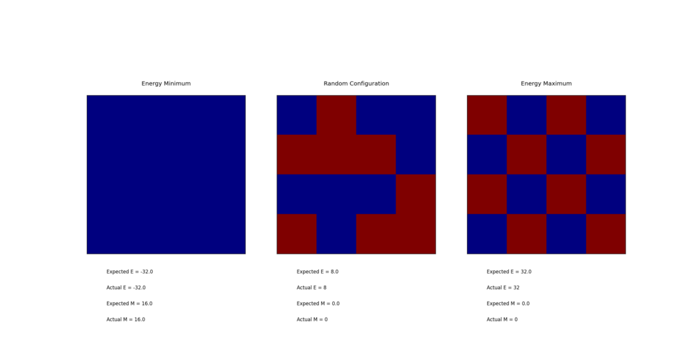
The energy for a random system of spins was modeled and compared to 'actual values' using the python module 'ILcheck.py'.
Originally, a system of for loops was built to run through the lattice and test each interaction 'forwards'. By forwards, scan the lattice left to right for rows, and top to bottom for columns and interactions were the product of the two spins. To adjust for periodic boundary conditions, at the final row/column, these values were multiplied by the values in the first column. This code is printed below:
   def energy(self):
       multiplied_spins = []
       for i in range(self.n_rows):
           for j in range(self.n_cols): #scan across (i,j): (0,0), (0,1).. (0, n), (1,0), (1,1),... (1,n)....(n,n)
               if (j+1) == self.n_cols: #If you're in the last column
                  multiplied_spins.append(2*self.lattice[i,j]*self.lattice[i,0]) #multiply the last column with the first row
               else:
                   multiplied_spins.append(2*self.lattice[i,j]*self.lattice[i,j+1]) #multiply the column with the consecutive column
               if (i+1) == self.n_rows: #same for rows
                   multiplied_spins.append(2*self.lattice[i,j]*self.lattice[0,j])
               else:
                   multiplied_spins.append(2*self.lattice[i,j]*self.lattice[i+1,j])
       energy = -0.5*np.sum(multiplied_spins)
       return energy
TASK: Run the ILcheck.py script from the IPython Qt console using the command
Introduction to Monte Carlo simulation
TASK: How many configurations are available to a system with 100 spins? To evaluate these expressions, we have to calculate the energy and magnetisation for each of these configurations, then perform the sum. Let's be very, very, generous, and say that we can analyse 1E9 configurations per second with our computer. How long will it take to evaluate a single value of ?
For a system containing 100 spins, there should be 2100 configurations of that system which should take, assuming a computer can calculate 1E9 configurations per second, 4.0196937E13 years using the above equations. This is very large and therefore and different way of calculating the average energy and magnetisation is required.
Only considering values of the boltzmann that are not 'vanishingly small' leads us to use our monte carlo cycles to only sample the populations the system is likely to occupy.
TASK: Implement a single cycle of the above algorithm in the montecarlocycle(T) function. This function should return the energy of your lattice and the magnetisation at the end of the cycle. You may assume that the energy returned by your energy() function is in units of ! Complete the statistics() function. This should return the following quantities whenever it is called: , and the number of Monte Carlo steps that have elapsed.
   def montecarlostep(self, T):
       energy0 = self.energy() #define energy 0 as being the original energy
       alpha0 = self.lattice #define alpha 0 as being the original lattice configuration
       random_i = np.random.choice(range(0, self.n_rows))
       random_j = np.random.choice(range(0, self.n_cols)) #assigns a random spin coordinate to the variables random_i and random_j
       self.lattice[random_i, random_j] = - self.lattice[random_i, random_j] #flip the spin
       alpha1 = self.lattice #assigning the lattice with the spin flipped to the variable alpha1
       energy1 = self.energy() #calling the new energy on the lattice with the flipped spin
       deltaE = energy1 - energy0 #finding the change in energy on flipping the spin
       if deltaE <= 0: #the monte carlo specifications
           alpha0 = alpha1
           energy0 = energy1
           self.lattice = alpha0
           magnetisation = self.magnetisation()
           energy = energy0
       else:
           random_number = np.random.random() #calculate R values
           boltzmann = np.exp(-deltaE/T)
           if random_number <= boltzmann:
               alpha0 = alpha1
               energy0 = energy1
               self.lattice = alpha0
               magnetisation = self.magnetisation()
               energy = energy0
           else:
               self.lattice = alpha0
               self.lattice[random_i, random_j] = - self.lattice[random_i, random_j] # Revert the spin
               magnetisation = self.magnetisation()
               energy = energy0
       self.n_cycles += 1 #Ensure that n_cycles is updated
       self.E += energy
       self.E2 += energy ** 2
       self.M += magnetisation
       self.M2 += magnetisation ** 2 # update the E/E2/M/M2 variables
       return energy, magnetisation
   def statistics(self):
       n_cycles = self.n_cycles #Useful to define n_cycles for future neglect of relaxation data
       aveE = 0.0
       aveE2 = 0.0
       aveM = 0.0
       aveM2 = 0.0 #These variables were kept- I know that I could have just defined aveE e.t.c below by using = instead of += but I kept the same form (I didn't really see a preference either way!)
       aveE += self.E /n_cycles
       aveE2 += self.E2/n_cycles
       aveM += self.M/n_cycles
       aveM2 += self.M2/n_cycles #Calculate the averages
       return aveE, aveE2, aveM, aveM2, self.n_cycles
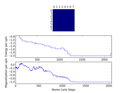
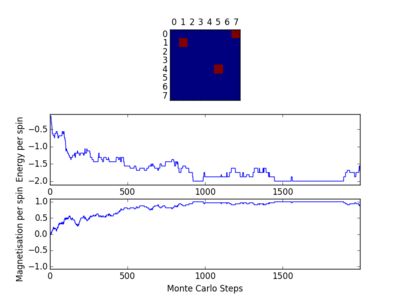
TASK: If T < Tc, do you expect a spontaneous magnetisation (i.e. do you expect )? When the state of the simulation appears to stop changing (when you have reached an equilibrium state), use the controls to export the output to PNG and attach this to your report. You should also include the output from your statistics() function.
Below the Curie temperature, by the definition of the Curie temperature, the critical point at which a spin/spins will swap, all spins will be parallel.
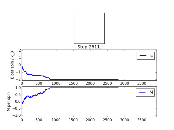
E = -1.88870362651
E*E = 3.64822093841
M = 0.913121352647
M*M = 0.881950120819
Accelerating the code
TASK: Use the script ILtimetrial.py to record how long your current version of IsingLattice.py takes to perform 2000 Monte Carlo steps. This will vary, depending on what else the computer happens to be doing, so perform repeats and report the error in your average!
3.397633s
Standard error: 0.005189532
TASK: Look at the documentation for the NumPy sum function. You should be able to modify your magnetisation() function so that it uses this to evaluate M. The energy is a little trickier. Familiarise yourself with the NumPy roll and multiplyfunctions, and use these to replace your energy double loop (you will need to call roll and multiply twice!).
   def energy(self):
       lattice = self.lattice #define a variable for the original lattice
       roll_rows_lattice = np.roll(lattice, 1, axis = 0) #shift the rows by 1 place in the original lattice
       multiply_rows = np.multiply(lattice,roll_rows_lattice) #multiply the original lattice with the rolled lattice, element wise
       roll_cols_lattice = np.roll(lattice, 1, axis = 1) #shift the columns by 1 place in the original lattice
       multiply_cols = np.multiply(lattice, roll_cols_lattice) #multiply the original lattice with the rolled lattice, element wise
       sum_everything = np.sum(multiply_rows) + np.sum(multiply_cols) #sum the interactions
       energy = -sum_everything #because this method has simulated the interactions on left to right/top to bottom or vice versa, i.e. in one direction, the 0.5 has been removed from the equation
       return energy
TASK: Use the script ILtimetrial.py to record how long your new version of IsingLattice.py takes to perform 2000 Monte Carlo steps. This will vary, depending on what else the computer happens to be doing, so perform repeats and report the error in your average!
0.135127s
Standard error: 0.001119
The effect of temperature
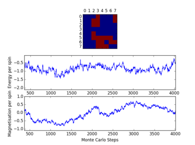
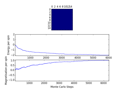
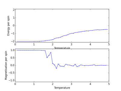
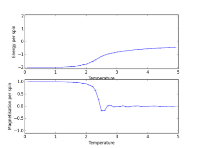
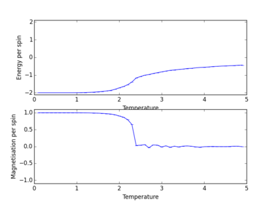
TASK: The script ILfinalframe.py runs for a given number of cycles at a given temperature, then plots a depiction of the final lattice state as well as graphs of the energy and magnetisation as a function of cycle number. This is much quicker than animating every frame! Experiment with different temperature and lattice sizes. How many cycles are typically needed for the system to go from its random starting position to the equilibrium state? Modify your statistics() and montecarlostep() functions so that the first N cycles of the simulation are ignored when calculating the averages. You should state in your report what period you chose to ignore, and include graphs from ILfinalframe.py to illustrate your motivation in choosing this figure.
| 16x16 | 32x32 |
|---|---|
 |
 |
| Lattice Size | Number of neglected data |
|---|---|
| 2x2 | 500 |
| 4x4 | 1000 |
| 8x8 | 2000 |
| 16x16 | 20000 |
| 32x32 | 50000 |
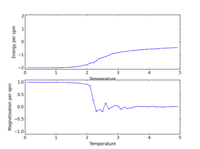
TASK: Use ILtemperaturerange.py to plot the average energy and magnetisation for each temperature, with error bars, for an 8x8 lattice. Use your initution and results from the script ILfinalframe.py to estimate how many cycles each simulation should be. The temperature range 0.25 to 5.0 is sufficient. Use as many temperature points as you feel necessary to illustrate the trend, but do not use a temperature spacing larger than 0.5. T NumPy function savetxt() stores your array of output data on disk — you will need it later. Save the file as 8x8.dat so that you know which lattice size it came from.
The effect of system size
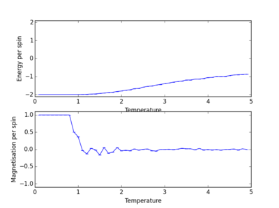
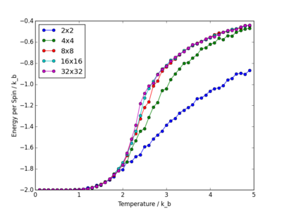
TASK: Repeat the final task of the previous section for the following lattice sizes: 2x2, 4x4, 8x8, 16x16, 32x32, 128x128. Make sure that you name each datafile that your produce after the corresponding lattice size! Write a Python script to make a plot showing the energy per spin versus temperature for each of your lattice sizes. Hint: the NumPy loadtxt function is the reverse of the savetxt function, and can be used to read your previously saved files into the script. Repeat this for the magnetisation. As before, use the plot controls to save your a PNG image of your plot and attach this to the report. How big a lattice do you think is big enough to capture the long range fluctuations?
 |
 |
 |
 |
 |
The standard errors do change (may be very small!)
Plotting energy vs temperature for the different system sizes:
Plot Magnetisation vs temperature for the different system sizes :
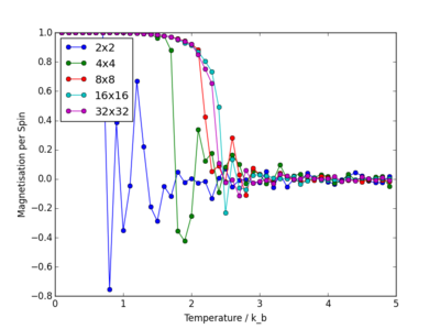
How big a lattice do you think is big enough to capture the long range fluctuations? The 8x8 is the smallest lattice size run that appears to energetically converge on the more accurate 16x16 and 32x32 lattice sizes.
Determining the heat capacity
TASK: Write a Python script to make a plot showing the heat capacity versus temperature for each of your lattice sizes from the previous section. You may need to do some research to recall the connection between the variance of a variable, , the mean of its square , and its squared mean . You may find that the data around the peak is very noisy — this is normal, and is a result of being in the critical region. As before, use the plot controls to save your a PNG image of your plot and attach this to the report.
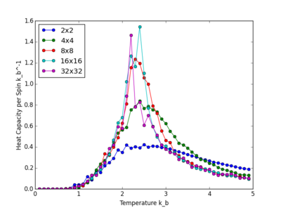
Locating the Curie temperature
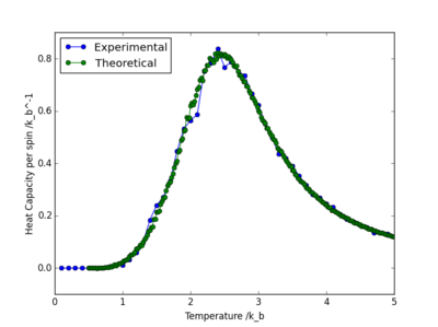
TASK: A C++ program has been used to run some much longer simulations than would be possible on the college computers in Python. You can view its source code here if you are interested. Each file contains six columns: (the final five quantities are per spin), and you can read them with the NumPy loadtxt function as before. For each lattice size, plot the C++ data against your data. For one lattice size, save a PNG of this comparison and add it to your report — add a legend to the graph to label which is which. To do this, you will need to pass the label="..." keyword to the plot function, then call the legend() function of the axis object (documentation here).
The PNG for one lattice size:
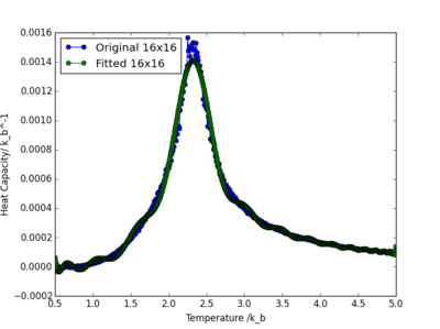
TASK: write a script to read the data from a particular file, and plot C vs T, as well as a fitted polynomial. Try changing the degree of the polynomial to improve the fit — in general, it might be difficult to get a good fit! Attach a PNG of an example fit to your report.
   import numpy as np
   from matplotlib import pylab as pl
   data = np.loadtxt("M16x16.dat") #load the txt contained within the file specified, and store it in the variable data
   T = data[:,0] #Temperatures stored in the first column of the .txt file will be stored in the T variable
   C = (data[:,2] - data[:,1]**2) / ((data[:,0]**2)*4) #Calculate the heat capacities of my data or use your data and specify C = data[:,5] (I was using my own data at this point and used yours later! The Curie temperatures were compared)
   fit = np.polyfit(T,C,10) #Perform a fit of the tenth order on the data
   T_min = np.min(T) #Find the minimum value in the temperatures defined by the variable T
   T_max = np.max(T) #Find the maximum value in the temperatures
   peak_T_range = np.linspace(T_min, T_max, 1000) #create an array of 1000 equally spaced data between T_min and T_max
   fitted_C_values = np.polyval(fit, peak_T_range) #Evaluate the polynomial at different values of peak_T_range
   g1, =pl.plot(T, C, 'o-', label = 'Original 16x16') #Plot the original data and label the data 'Original *insert lattice size here*'
   g2, =pl.plot(peak_T_range, fitted_C_values, 'o-', label = 'Fitted 16x16') #plot the fitted data
   pl.legend(handles = [g1,g2], loc=2) #Add the legend
   pl.xlabel('Temperature')
   pl.ylabel('Heat Capacity') #label x and y
   pl.show()
TASK: Modify your script from the previous section. You should still plot the whole temperature range, but fit the polynomial only to the peak of the heat capacity! You should find it easier to get a good fit when restricted to this region.
   import numpy as np
   from matplotlib import pylab as pl
   data = np.loadtxt("M16x16.dat")
   T = data[:,0]
   C = (data[:,2] - data[:,1]**2) / ((data[:,0]**2)*4)
   fit = np.polyfit(T,C,400)
   Tmin = 2.1
   Tmax = 2.55 #Define Tmin and Tmax
   selection = np.logical_and(T > Tmin, T < Tmax) #Use the numpy logical_and function to find the indices that return the Boolean 'True'
   peak_T_values = T[selection]
   peak_C_values = C[selection] # Use these indexed boolean values to refine our data set between Tmin and Tmax
   T_min = np.min(peak_T_values)
   T_max = np.max(peak_T_values)
   peak_T_range = np.linspace(T_min, T_max, 1000)
   fitted_C_values = np.polyval(fit, peak_T_range)
   g1, =pl.plot(T, C, 'o-', label = 'Original 32x32')
   g2, =pl.plot(peak_T_range, fitted_C_values, 'o-', label = 'Fitted 32x32')
   pl.legend(handles = [g1,g2], loc=2)
   pl.xlabel('Temperature /Reduced units')
   pl.ylabel('Heat Capacity/ k_b')
   pl.show()
   Cmax = np.max(fitted_C_values)
   Tmax = peak_T_range[fitted_C_values == Cmax]
   print(Tmax)
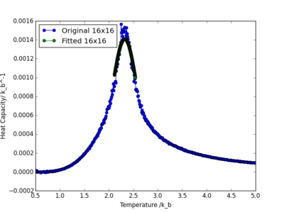
TASK: find the temperature at which the maximum in C occurs for each datafile that you were given. Make a text file containing two colums: the lattice side length (2,4,8, etc.), and the temperature at which C is a maximum. This is your estimate of for that side length. Make a plot that uses the scaling relation given above to determine . By doing a little research online, you should be able to find the theoretical exact Curie temperature for the infinite 2D Ising lattice. How does your value compare to this? Are you surprised by how good/bad the agreement is? Attach a PNG of this final graph to your report, and discuss briefly what you think the major sources of error are in your estimate.
Performing the linear fit for your data in the figure below gave a Curie Temperature
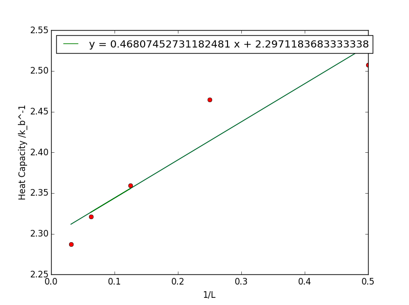
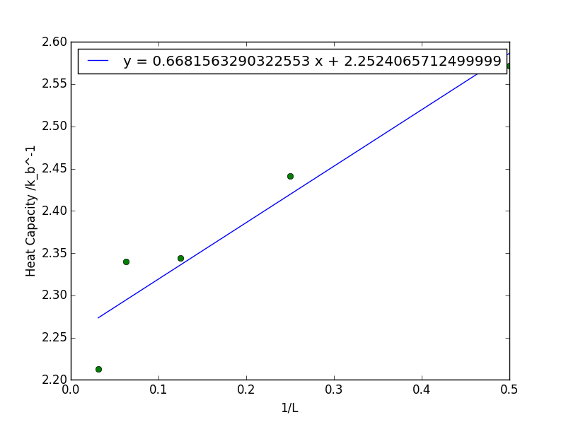
The Curie temperature of the infinite lattice obtained for both the calculation on the given data and the Curie temperature of the infinite lattice obtained for the data generated were found to be 2.30 and 2.25. 2.25 was closer to the literature value 1 reported to be 2.269. The major sources of error were most likely computational inconsistency and the monte carlo method is only an approximation and based on random generation of data. I am surprised at the accuracy of the calculation- the approximations used have saved 4.0196937E13 years of computational time, which I believe is an added bonus. Putting it into perspective, the universe is only 13.8 billion years old and the calculation would take 40196.937 billion years. Thank you Monte Carlo!
References
1) http://www.physics.buffalo.edu/phy410-505/2011/topic5/app2/

