Rep:Mod:mpg15CMP

Section 1

Task 1: The energy of the Isling model

The interaction energy is defined by the equation: $$\begin{gathered} E \\ =-\frac{1}{2}J\sum _i^N\sum _{j \\ \in \\ \mathrm{n}\mathrm{e}\mathrm{i}\mathrm{g}\mathrm{h}\mathrm{b}\mathrm{o}\mathrm{u}\mathrm{r}\mathrm{s}\left(i\right)}{s}_i{s}_j \end{gathered}$$. The number of adjacent neighbours of each cell is equal to 2xD, where D is the number of dimensions of the cell. To find the minimum point, we take the case where all $s_i$ have the same spin, which results in the first sum being simply 2D. We are left with the equation: $$\begin{gathered} E \\ =-\frac{1}{2}J\sum _i^{N}2D \end{gathered}$$, which is equivalent to $$\begin{gathered} E \\ = \\ -DNJ \end{gathered}$$.

This state has a multiplicity of two, as it can exist with all spins +1, or all spins -1.

To calculate the entropy, we use the equation: $S=k_{\mathrm{B}}\ln \mathrm{\Omega }$. Since we have two possible states, $S=9.572\times 10^{-24}J{K}^{-1}$

Task 2: Energy Change

Since D=3 and N=1000, E=-3000J in the initial case. When one of the spins flips, one s_is_j interaction changes sign, so the energy becomes $$\begin{gathered} E \\ =-\frac{1}{2}J\times 6\times ((999\times 1)-1) \end{gathered}$$, which is equivalent to -2994J. $\mathrm{△}E=+6J$

The value of $\mathrm{\Omega }$ increases to 2000 in this situation, so the entropy increases to $S=1.050\times 10^{-22}J{K}^{-1}$

Task 3: Magnetisation of the Lattice

The magnetisation of the lattice is $M=\sum _i{s}_i$. For the one dimensional lattice, $M=3-2=1$. For the two dimensional lattice, $M=13-12=1$.

At absolute zero, we would assume the lattice to have the lowest energy configuration, with all the spins parallel. Since $N=1000,M=1000$

Section 2

Task 1: Energy and Magnetisation functions

The code used in the Energy function is as follows:

def energy(self):
       "Return the total energy of the current lattice configuration."
       in_sum=0
       
       for i in range(len(self.lattice)):
           if i < self.n_rows -1:
               for j in range(len(self.lattice)):
                   if j < self.n_rows -1:
                       si=self.lattice[i,j]
                       sj_x=self.lattice[i+1,j]
                       sj_y=self.lattice[i,j+1]
                       in_x=si*sj_x
                       in_y=si*sj_y
                       in_sum=in_sum+in_x+in_y
                   if j == self.n_rows -1:
                       si=self.lattice[i,j]
                       sj_x=self.lattice[i+1,j]
                       sj_y=self.lattice[i,0]
                       in_x=si*sj_x
                       in_y=si*sj_y
                       in_sum=in_sum+in_x+in_y
           if i == self.n_rows -1:
               for j in range(len(self.lattice)):
                   if j < self.n_rows-1:
                       si=self.lattice[i,j]
                       sj_x=self.lattice[0,j]
                       sj_y=self.lattice[i,j]
                       in_x=si*sj_x
                       in_y=si*sj_y
                       in_sum=in_sum+in_x+in_y
                   if j == self.n_rows-1:
                       si=self.lattice[i,j]
                       sj_x=self.lattice[0,j]
                       sj_y=self.lattice[i,0]
                       in_x=si*sj_x
                       in_y=si*sj_y
                       in_sum=in_sum+in_x+in_y
       energy = in_sum
       return energy

The code used for the magnetisation function is as follows:

   def magnetisation(self):
       "Return the total magnetisation of the current lattice configuration."
       magnetisation = np.sum(self.lattice)
       return magnetisation

Task 2: Ising Lattice Check

The lattice check was performed successfully, with the code giving the expected outputs:

Lattice Check

Section 3

Task 1: 100 Spin System configuration

For the 100 spin system, the number of configurations $\mathrm{\Omega }=2^{100}=1.268\times 10^{30}$

If we can sum $10^9$ configurations per second, sampling all of these will take $1.268\times 10^{21}s$: 400 trillion years!

Task 2: Monte Carlo Step

The code for the single Monte Carlo simulation step is:

   def montecarlostep(self, T):
       # complete this function so that it performs a single Monte Carlo step
       a1=self.lattice
       e1=self.energy
       random_i = np.random.choice(range(0, self.n_rows))
       random_j = np.random.choice(range(0, self.n_cols))
       for i in range(len(self.lattice)):
           for j in range(len(self.lattice)): 
               if i == random_i and j == random_j:
                   self.lattice[i,j]=self.lattice[i,j]*-1
       if self.energy() < e1():
           self.lattice = self.lattice
       if self.energy() > e1():
           random_number = np.random.random()
           probability = np.exp(-(self.energy-e1)/T*(1.38064852*10**-23))
           if random_number <= probability:
               self.lattice = self.lattice
           if random_number > probability:
               self.lattice = a1			
       self.E = self.E+self.energy()
       self.E2 = self.E2+(self.energy())**2
       self.M = self.M+self.magnetisation()
       self.M2 = self.M2+(self.magnetisation())**2
       self.n_cycles = self.n_cycles+1
       return(self.energy(), self.magnetisation())

The code for the statistics function is as follows:

   def statistics(self):
       avE=self.E/(self.n_cycles+1)
       avE2=self.E2/(self.n_cycles+1)
       avM=self.M/(self.n_cycles+1)
       avM2=self.M2/(self.n_cycles+1)
       # complete this function so that it calculates the correct values for the averages of E, E*E (E2), M, M*M (M2), and returns them
       return(avE,avE2,avM,avM2)

Task 3: Simulation Output

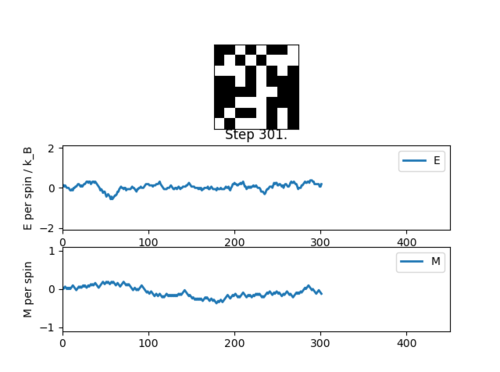
The simulation essentially starts at equillibrium, with small variations visible throughout:

Simulation Output

The number outputs from the statistics() function are as follows:

Section 4

Task 1: Original Calculation Time

The results of the initial run of the timetrial function are as follows:

Trial 1	7.351s
Trial 2	7.326s
Trial 3	7.492s
Trial 4	7.308s
Av.Time	7.369s

Task 2: Optimising Code

The original magnetism function already used the np.sum() method. The energy calculation code was improved to now read:

def energy(self):
       xmult=np.multiply(self.lattice, np.roll(self.lattice,-1,axis=1))
       ymult=np.multiply(self.lattice, np.roll(self.lattice,-1,axis=0))
       tot=np.sum(xmult)+np.sum(ymult)
       energy=tot*-1
       return energy

Task 3: Optimised Calculation Time

The results of the second run of the timetrial function are as follows:

Trial 1	0.421s
Trial 2	0.424s
Trial 3	0.422s
Trial 4	0.424s
Av.Time	0.423s

The use of the numpy roll() and multiply() functions has vastly reduced the time needed for each step.

Section 5

Task 1: Correcting the Averaging Code

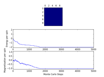
The number of steps necessary for the simulation to reach an equilibrium increased with the dimensions of the lattice. To account for this, the number of steps to ignore for the averaging, N, is going to be determined by the equation: $N=L^3\times 3$, where L is the length of the lattice.

5v5 Lattice	10v10 Lattice	15v15 Lattice	20v20 Lattice
N=375	N=3000	N=10125	N=24000

As shown in the table, equilibrium is reached for every lattice size before the value of N is reached.

The amended sections of code are as follows:

In the montecarlostep() function:

      if self.n_cycles > (len(self.lattice())**3)*3
           self.E+=self.energy()
           self.E2+=self.energy()**2
           self.M+=self.magnetisation()
           self.M2+=self.magnetisation()

In the statistics() function:

  def statistics(self):
       avE=self.E/(self.n_cycles-(len(self.lattice())**3)*3)
       avE2=self.E2/(self.n_cycles-(len(self.lattice())**3)*3)
       avM=self.M/(self.n_cycles-(len(self.lattice())**3)*3)
       avM2=self.M2/(self.n_cycles-(len(self.lattice())**3)*3)
       # complete this function so that it calculates the correct values for the averages of E, E*E (E2), M, M*M (M2), and returns them
       return(avE,avE2,avM,avM2)

Task 2: Range of Temperatures

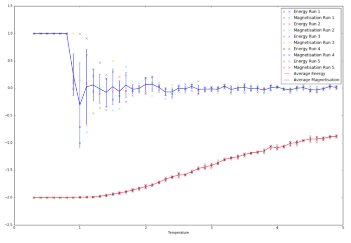
After some amendments to the code, the temperature range simulation was ran a total of 5 times for 100,000 steps. The large number of steps was chosen to make sure the data was accurate, as smaller step counts would show significant fluctuations. It is clear from the graph that the data showed very little variance in between repeats at the two ends of the temperature range, where either the high or low temperature configuration was achieved.

Significant noise is visible in the 1.7-3.5 degree range, especially in the magnetism plot, as shown by the large error bars. The energy function also shows slightly increased variation around that temperature range, although the error bars remain small enough to be essentially invisible.

This noise is likely caused by the fact this region is in between the high and low energy states, leaving the system in a much more randomised configuration. Since its not driven to either the low or high energy state (or the corresponding high or low magnetism state), the system can end up with very different average energies at the end of the simulation.

8x8 Lattice Temperature range

Section 6

Task 1: Scaling the System Size

Looking at the results for the range of lattice sizes, it is clear that the accuracy of the simulation increases with the increase of lattice size, with the phase transition region smoothing out and showing a reduction in the noise. The two smallest lattices are quite inadequate in showing the behaviour of the system, especially in the 1-2 degree range, where they show wild variation across the repeats. As the lattice size was increased, so was the number of steps taken in the simulation to allow for the increased time to reach equilibrium. 10000 steps were used for 2v2, 40,000 for 4v4, 100,000 for 8v8, 500,000 for 16v16, and 800,000 for 32v32 (at which point the calculation ran for the best part of an hour). To increase the accuracy of the calculated values the number of skipped steps was increased to $N=L^3\times 4$, as some of the lattices showed problems with very large errors in the calculation.

Average Energy Calculations

2x2 Lattice	4x4 Lattice

8x8 Lattice	16x16 Lattice

32x32 Lattice

Section 7

Task 1: Derivation of Heat Capacity Equation

To get to the desired definition of heat capacity, we start with the partition function: $Z=\sum _i\exp \{-\frac{E\left(\alpha \right)}{k_{B}T}\}$ and the definition of heat capacity: $C=\frac{\partial ⟨E⟩}{\partial T}$

We know that the average energy of the system is equal to: ${⟨E⟩}_T=\frac{1}{Z}\sum _{\alpha }E\left(\alpha \right)\exp \{-\frac{E\left(\alpha \right)}{k_{B}T}\}$

Which equals: ${⟨E⟩}_T=-\frac{1}{Z}\frac{\partial Z}{\partial \beta }$ where $\beta =\frac{1}{k_{B}T}$

Which equals: ${⟨E⟩}_T=\frac{\partial Ln(Z)}{\partial \beta }$

Taking the following expressions: $\mathrm{V}\mathrm{a}\mathrm{r}[E]=⟨E^2⟩-{⟨E⟩}^2$ and $⟨E^2⟩=\frac{{\partial }^{2}Z}{\partial {\beta }^2}$

We can see that: $\mathrm{V}\mathrm{a}\mathrm{r}[E]=\frac{{\partial }^{2}Ln(Z)}{\partial {\beta }^2}$

Which is equivalent to: $\mathrm{V}\mathrm{a}\mathrm{r}[E]=-\frac{\partial T}{\partial \beta }\times \frac{\partial ⟨E⟩}{\partial T}=k_B{T}^{2}C$

This finally rearranges to: $C=\frac{\mathrm{V}\mathrm{a}\mathrm{r}[E]}{k_B{T}^2}$, which is the desired equation.

Task 2: Heat Capacity Plots

The code used to determine the heat capacity for each lattice size is as follows:

def multicapacity(data1,data2,data3,data4,data5, spin):

   t1=data1[:,0]
   e1=data1[:,1]
   e21=data1[:,2]

   t2=data2[:,0]
   e2=data2[:,1]
   e22=data2[:,2]

   t3=data3[:,0]
   e3=data3[:,1]
   e23=data3[:,2]

   t4=data4[:,0]
   e4=data4[:,1]
   e24=data4[:,2]

   t5=data5[:,0]
   e5=data5[:,1]
   e25=data5[:,2]
      
   n=spin**2
   
   ave=(e1+e2+e3+e4+e5)/5
   ave2=(e21+e22+e23+e24+e25)/5

   figure(figsize=[9,6])
   
   plot(t1, (abs(e21-(e1**2))/t1**2)/n, label="Run 1", linestyle = , marker='x')
   plot(t2, (abs(e22-(e2**2))/t2**2)/n, label="Run 2" ,linestyle = , marker='x')
   plot(t3, (abs(e23-(e3**2))/t3**2)/n, label="Run 3",linestyle = , marker='x')
   plot(t4, (abs(e24-(e4**2))/t4**2)/n, label="Run 4",linestyle = , marker='x')
   plot(t5, (abs(e25-(e5**2))/t5**2)/n, label="Run 5",linestyle = , marker='x')
   plot(t1, (abs(ave2-(ave**2))/t1**2)/n, label = "Average", color='red',linestyle="--", linewidth="2")
   legend(loc="upper right")
   xlabel("Temperature")
   show()
   return(ave, ave2,t1)

As you can see the data shows relatively small variations throughout the range of temperatures, with the greatest noise appearing around the peak. The general shape of the plot is caused by the fact the system undergoes a phase transition within the range of temperatures, at which point the heat capacity rises greatly as the energy of the system goes towards reorganisation.

8x8 Lattice Heat Capacities

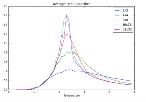
The plot of all the heat capacities was made using the average heat capacities calculated for each set of five lattices. The increasingly sharp and tall peak of the curves corresponds to the narrower and steeper phase transition region for the larger systems. The very small difference between the 16x16 and 32x32 systems shows that the 16x16 lattice is the smallest lattice size past which no real changes are visible in the calculated data.

All Lattice Heat Capacities

Section 8

Task 1: C++ Data Comparison

The 8x8 Lattice was taken as an example of the difference in between the results calculated using python and the given files. As you can see the two data sets are a very good match, with the only visible difference being the very slight shift of the python curve to the left.

8x8 C++/Python Comparison

Task 2: Fitted Data to C++

The code used to fit a curve to the C++ data is as follows:

def Capacity(data):

   T=data[:,0]
   C=data[:,5]
   fit = np.polyfit(T, C, 100)
   T_min = np.min(T)
   T_max = np.max(T)
   T_range = np.linspace(T_min, T_max, 1000) 
   fitted_C_values = np.polyval(fit, T_range) 
   plot(T_range, fitted_C_values,label="Fitted Polynomial of order 100", linewidth=2, color="red")
   plot(T,C, label = "Raw Data", linestyle='--', color = "green")
   legend(loc="lower right")
   show()

The polynomial used is of a very high degree. This was essentially the highest polynomial that showed any significant difference in the accuracy of the fit, as lower-order polynomials significantly underestimated the value of the peak of the graph. This fit still falls quite significantly short, however.

32x32 C++ Poor Fit

Task 3: Restricted Fit

The code used in the restricted fit is as follows:

def Capacity(data):

   T=data[:,0]
   C=data[:,5]
   points=len(T)
   point_min=round(points*0.25)
   point_max=round(points*0.6)
   T2=data[point_min:point_max,0]
   C2=data[point_min:point_max,5]
   fit = np.polyfit(T2, C2, 100)
   T_min2 = np.min(T2)
   T_max2 = np.max(T2)
   T_range2 = np.linspace(T_min2, T_max2, 1000) 
   fitted_C_values = np.polyval(fit, T_range2) 
   
   figure(figsize=[9,6])
   plot(T_range2, fitted_C_values,label="Fitted Polynomial of order 100", linewidth=2, color="red")
   plot(T,C, label = "Raw Data", linestyle='--', color = "green")
   legend(loc="lower right")
   title("Improved Fitting to C++ Data")
   show()
   Cmax = np.max(fitted_C_values)
   Tmax =T_range2[fitted_C_values == Cmax]

   return (Cmax, Tmax[0])

The method used to restrict the code is somewhat different from the one suggested, but it gives the same result. The fit is now much better, representing the shape of the peak almost perfectly.

32x32 C++ Good Fit

Task 4: Finding Tc

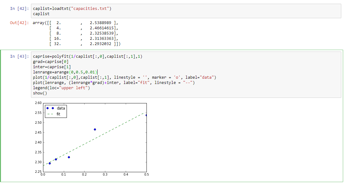
The code used and the plot of the heat capacity graph is below, with "caplist" being a handmade list of the maximum heat capacities from the C++ files as outputted by the code above:

Fit of C values

The fitted data shows a reasonably linear trend, with the intercept giving the infinite-lattice heat capacity as 2.281. This is fairly close to the literature value of 2.269. The fluctuations within the data and its difference from the literature could be caused by a number of factors. One is the rather small data set used for the fit - more data points would be needed, especially from lattice sizes larger than 32x32. The variation of the lower lattice sizes from the fit can be explained by the fact the lattice itself is not of an adequate size to give a reasonable value for the heat capacity, as shown by the very wide peaks in the plots of the python data. Another possible source of error could come from the random number used in the monte carlo simulation. Since the randomness of this value underpins the very principles of the process, the method used by Python or C++ to generate these could have an impact on the accuracy of the data.

References

- ↑ L. Onsager, Physical Review, 1944, 65, 117