Rep:Mod:mh3413Liquids

Molecular dynamics simulations of simple liquids

Abstract

This experiment explored the molecular dynamics of the isothermal–isobaric (N,P,T) and the canonical (N,V,T) thermodynamic ensemble in a solid, liquid and gaseous phase over time. By exploring the Lennard-Jones Potential energy surface, through the interactions of the particles, an appropriate cut-off value for the molecular simulations were able to be determined. By applying the period boundary conditions to the unit cell, the number of atoms to remained constant and the unit cells were ‘linked’. The total energy for different timesteps were used to determine a timestep value that would maximise the time of the system simulation, while also maximising the detail of the system captured. In addition, the energy timestep plots allowed the determination of the systems that had reached thermodynamic equilibrium in a appropriate number of timesteps. Using this knowledge of the LAMMPS and VMD platform, the thermodynamics properties for solid, liquid and gaseous states were successfully investigated. Physical constants such as the diffusion co-efficient were able to be approximated. This required steps of selecting physical parameters for the system eg number density, number of unit cells in the lattice, and then applying the system conditions to melt the lattice to the required temperature and state. The following sections will explain in detail the rational and steps taken for each of the calculations undertaken.

Task 2 - Velocity Verlet Algorithm

TASK: Open the file HO.xls. In it, the velocity-Verlet algorithm is used to model the behaviour of a classical harmonic oscillator. Complete the three columns "ANALYTICAL", "ERROR", and "ENERGY": "ANALYTICAL" should contain the value of the classical solution for the position at time $t$, "ERROR" should contain the absolute difference between "ANALYTICAL" and the velocity-Verlet solution.

molecule1	molecule1
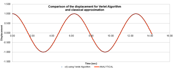
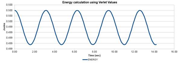
Figure 1: The values of the classical and Verlet displacement approximation for a timestep of 0.1	Figure 2: The total energy of the harmonic oscillator for a timestep of 0.1

Figure 3: Errors of the Velocity-Verlet algorithm relative to the classical approximation for a timestep of 0.1

Figure 4: The values of the maximas in the errors and the corresponding time for a timestep of 0.1

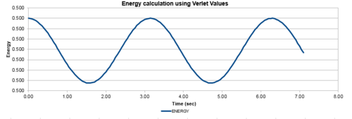
In this section, the calculated values of particle position from the Velocity-Verlet algorithm were compared to the values of the classical harmonic oscillator. The classical harmonic oscillator position at time t was given by $x\left(t\right)=A\cos (\omega t+\varphi )$, where the values of $A$ and $\omega$ were all assumed to be equal to 1, while $\varphi =0$. Figure 1, illustrates the ideal fit of the data between the Velocity-Verlet algorithm and classical value, while figure 2 calculated the total energy of the system. The total energy of the harmonic oscillator consisted of Kinetic and Potential energies. The kinetic energy was obtained by using the equation $$\begin{gathered} E_k=\frac{1}{2} \\ m \\ {v}^2 \end{gathered}$$, where mass had a value of 1 and the Velocity-Verlet algorithm values were used for the velocity. The potential energy was calculated from 1-D harmonic oscillator $$\begin{gathered} E=\frac{1}{2} \\ k \\ {x}^2 \end{gathered}$$ where the x value was the displacement from the equilibrium distance. The oscillating nature originated from the exchange of potential and kinetic energy in the system, with relatively minimal changes in the total energy.

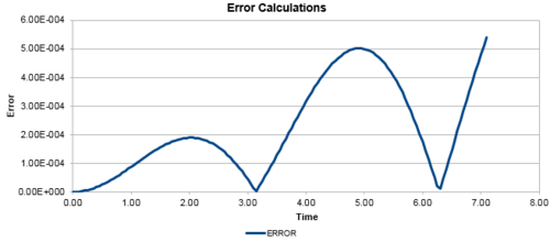
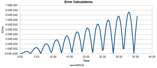
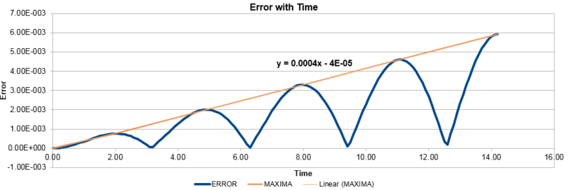
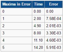
In addition, the difference between the values of the Velocity-Verlet algorithm values for position and the classical position for the harmonic oscillator as seen above, was plotted against time in figure 3. In a similar behaviour to the displacement and the energy, the error oscillates as the error is 0 for some values of t. However, the error does not fall below 0. With increasing time, the error associated with the Velocity-Verlet algorithm values relative to the classical harmonic oscillator increased in value. The equation for the approximated linear relationship between the maxima's of the errors with time can been seen in figure 4.

molecule1	molecule1	molecule1
Figure 5: Total Energy for the system at a timestep of 0.01	Figure 6: Total Energy for the system at a timestep of 0.05	Figure 7: Total Energy for the system at a timestep of 0.25

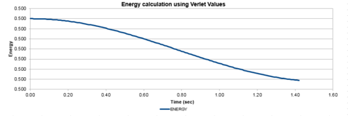
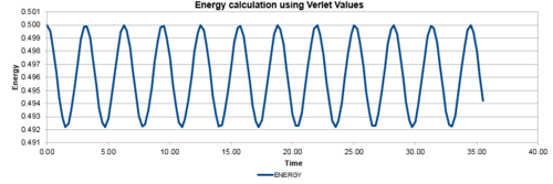
Experimenting with different values of timesteps to calculate the total energy (figures 5-7) and the total error (figures 8-10), it was found that the error of the maxima (ie the amplitude of the oscillations) increased with an increasing value in the timestep. There was a linear relationship between the maxima's of the errors with respect to time. At the timestep of 0.25, the fluctuation of the error was observed to be approx 1.6%. At a timestep value of 0.05, the fluctuations in the total energy for the system did not change to 3dp, while still maintaining the oscillation nature of the system. Through a trial and error method, a suitable timestep to ensure that the total energy does not change by more than 1% was found to be t=0.20. Any timestep value less than t=0.2 would be suitable for the purposes of the calculations. However, the shorter timestep would result in a shorter simulation of the system. This could be compensated by increasing the number of runs for the system, but this would require greater computational power.

The total energy is a strong indicator as to whether the system is at thermodynamic equilibrium. If the total energy has not equilibrated, then the other physical properties observed would likely be different to the ones observed at thermodynamic equilibrium.

molecule1	molecule1	molecule1
Figure 8: Total Error for the system at a timestep of 0.01	Figure 9: Total Error for the system at a timestep of 0.05	Figure 10: Total Error for the system at a timestep of 0.25

Lennard-Jones Potential

The Lennard-Jones Potential describes the potential of a system as two atoms or molecules approach one another from a large distance. The weak interactions between the particle species, of both repulsive and attractive forces will lead to the formation of an equilibrium distance, where the potential energy is minimised in a potential well. The repulsive component of ${\left(\frac{\sigma }{r_{ij}}\right)}^{12}$ is significant at short distances, where the term would be dominant. The attractive component of ${\left(\frac{\sigma }{r_{ij}}\right)}^6$ is dominant at large distances, and this is seen in the graph of the Lennard-Jones Potential as U tends towards 0 at very large values of r.

TASK: Find the separation, $r_0$, at which the potential energy is zero

$U(r^N)=\sum _i^N\sum _{i\ne j}^N=4\epsilon [{\left(\frac{\sigma }{r_{ij}}\right)}^{12}-{\left(\frac{\sigma }{r_{ij}}\right)}^6]$

$U(r^N)=0$

$0=[{\left(\frac{\sigma }{r_{ij}}\right)}^{12}-{\left(\frac{\sigma }{r_{ij}}\right)}^6]$

${\frac{\sigma }{r_{ij}}}^{12}={\frac{\sigma }{r_{ij}}}^6$

${\frac{\sigma }{r_{ij}}}^6=1$

${\sigma }^6=r_{ij}^6$

When $$\begin{gathered} \therefore \\ U(r^N)=0 \end{gathered}$$

SOLUTION: $$\begin{gathered} \therefore \\ {r}_{ij}=\sigma \end{gathered}$$ OR $$\begin{gathered} \therefore \\ {r}_{ij}=\mathrm{\infty } \end{gathered}$$

Therefore there are two solution to where the Lennard-Jones potential is U=0. At a value of r=infinity, the Lennard-Jones Potential will tend towards the U=0 value.

TASK: What is the force at this separation? As ${\mathbf{F}}_i=-\frac{\mathrm{d}U\left({\mathbf{r}}^N\right)}{\mathrm{d}{\mathbf{r}}_i}$

$U\left({\mathbf{r}}^N\right)=\sum _i^N\sum _{i\ne j}^N\left\{4ϵ(\frac{{\sigma }^{12}}{r_{ij}^{12}}-\frac{{\sigma }^6}{r_{ij}^6})\right\}$

${\mathbf{F}}_i=-\frac{\mathrm{d}\sum _i^N\sum _{i\ne j}^N\left\{4ϵ(\frac{{\sigma }^{12}}{r_{ij}^{12}}-\frac{{\sigma }^6}{r_{ij}^6})\right\}}{\mathrm{d}{\mathbf{r}}_i}$

${\mathbf{F}}_i=-\sum _i^N\sum _{i\ne j}^N\left\{4ϵ(\frac{-12{\sigma }^{12}}{r_{ij}^{13}}+\frac{6{\sigma }^6}{r_{ij}^7})\right\}$

As $\sigma =r_{ij}$ as $U(r^N)=0$

SOLUTION $\therefore {\mathbf{F}}_i=\frac{24ϵ}{\sigma }$

TASK: Find the equilibrium separation, $r_{eq}$

$U\left({\mathbf{r}}^N\right)=\sum _i^N\sum _{i\ne j}^N\left\{4ϵ(\frac{{\sigma }^{12}}{r_{ij}^{12}}-\frac{{\sigma }^6}{r_{ij}^6})\right\}$

$\frac{\mathrm{d}U\left({\mathbf{r}}^N\right)}{\mathrm{d}{\mathbf{r}}_i}=\sum _i^N\sum _{i\ne j}^N\left\{4ϵ(\frac{-12{\sigma }^{12}}{r_{ij}^{13}}+\frac{6{\sigma }^6}{r_{ij}^7})\right\}$

Let $\frac{\mathrm{d}U\left({\mathbf{r}}^N\right)}{\mathrm{d}{\mathbf{r}}_i}=0$ to find the stationary point (ie minimum) in the Lennard-Jones Potential.

$4ϵ(\frac{-12{\sigma }^{12}}{r_{ij}^{13}}+\frac{6{\sigma }^6}{r_{ij}^7})=0$

$\frac{6{\sigma }^6}{r_{ij}^7}=\frac{12{\sigma }^{12}}{r_{ij}^{13}}$

$1=\frac{2{\sigma }^6}{r_{ij}^6}$

$r_{eq}=2^{1/6}\sigma$

When $r_{eq}=2^{1/6}\sigma$

Then: $U\left({\mathbf{r}}_{eq}\right)=\sum _i^N\sum _{i\ne j}^N\left\{4ϵ(\frac{{\sigma }^{12}}{r_{eq}^{12}}-\frac{{\sigma }^6}{r_{eq}^6})\right\}=\sum _i^N\sum _{i\ne j}^N\left\{4ϵ(\frac{{\sigma }^{12}}{4{\sigma }^{12}}-\frac{{\sigma }^6}{2{\sigma }^6})\right\}$

$U\left({\mathbf{r}}_{eq}\right)=\sum _i^N\sum _{i\ne j}^N\left\{4ϵ(\frac{1}{4}-\frac{1}{2})\right\}$

SOLUTION: $$\begin{gathered} \therefore \\ U\left({\mathbf{r}}_{eq}\right)=-ϵ \end{gathered}$$ This is the value of the potential minimum in the Lennard-Jones Potential

TASK: Evaluate the integrals $\underset{2\sigma }{\overset{\mathrm{\infty }}{\int }}\varphi \left(r\right)\mathrm{d}r$, $\underset{2.5\sigma }{\overset{\mathrm{\infty }}{\int }}\varphi \left(r\right)\mathrm{d}r$, and $\underset{3\sigma }{\overset{\mathrm{\infty }}{\int }}\varphi \left(r\right)\mathrm{d}r$ when $\sigma =ϵ=1.0$.

The integral of the Lennard-Jones Potential corresponds to the the total interaction between the two species. As the lower limit approaches greater values of r, the total integral value tends to 0, as the Lennard-Jones Potential tends to infinity for larger values of r. In addition, the area of curve would be negative as the curve approaches 0 from the negative y values.

$\underset{2\sigma }{\overset{\mathrm{\infty }}{\int }}\varphi \left(r\right)\mathrm{d}r$

$\varphi \left(r\right)=4ϵ(\frac{{\sigma }^{12}}{r^{12}}-\frac{{\sigma }^6}{r^6})$

$\underset{2\sigma }{\overset{\mathrm{\infty }}{\int }}\varphi \left(r\right)\mathrm{d}r=\underset{2\sigma }{\overset{\mathrm{\infty }}{\int }}4ϵ(\frac{{\sigma }^{12}}{r^{12}}-\frac{{\sigma }^6}{r^6})\mathrm{d}r$

$$\begin{gathered} \underset{2\sigma }{\overset{\mathrm{\infty }}{\int }}\varphi \left(r\right)\mathrm{d}r=4ϵ(\frac{{\sigma }^{12}}{-11r^{11}}-\frac{{\sigma }^6}{-5r^5}){|}_{2\sigma }^{\mathrm{\infty }} \\ (1) \end{gathered}$$

$\underset{2\sigma }{\overset{\mathrm{\infty }}{\int }}\varphi \left(r\right)\mathrm{d}r=0-4ϵ(\frac{{\sigma }^{12}}{11\times {(2\sigma )}^{11}}-\frac{{\sigma }^6}{5\times {(2\sigma )}^5})$

$\underset{2\sigma }{\overset{\mathrm{\infty }}{\int }}\varphi \left(r\right)\mathrm{d}r=0-4ϵ(\frac{\sigma }{11\times {(2)}^{11}}-\frac{\sigma }{5\times {(2)}^5})$

$\underset{2\sigma }{\overset{\mathrm{\infty }}{\int }}\varphi \left(r\right)\mathrm{d}r=-4ϵ(\frac{\sigma }{22528}-\frac{\sigma }{160})$

$\underset{2\sigma }{\overset{\mathrm{\infty }}{\int }}\varphi \left(r\right)\mathrm{d}r=-ϵ\left(\frac{699\sigma }{28160}\right)=-0.0248224....$

when $\sigma =ϵ=1.0$

SOLUTION $\therefore \underset{2\sigma }{\overset{\mathrm{\infty }}{\int }}\varphi \left(r\right)\mathrm{d}r\approx -0.0248(3sf)$

From modification of equation 1: $$\begin{gathered} \underset{2.5\sigma }{\overset{\mathrm{\infty }}{\int }}\varphi \left(r\right)\mathrm{d}r=4ϵ(\frac{{\sigma }^{12}}{-11r^{11}}-\frac{{\sigma }^6}{-5r^5}){|}_{2.5\sigma }^{\mathrm{\infty }} \\ (1) \end{gathered}$$

$\underset{2.5\sigma }{\overset{\mathrm{\infty }}{\int }}\varphi \left(r\right)\mathrm{d}r=0-4ϵ(\frac{{\sigma }^{12}}{11\times {(2.5\sigma )}^{11}}-\frac{{\sigma }^6}{5\times {(2.5\sigma )}^5})$

$\underset{2.5\sigma }{\overset{\mathrm{\infty }}{\int }}\varphi \left(r\right)\mathrm{d}r=(-0.008176747....)$

SOLUTION$\therefore \underset{2.5\sigma }{\overset{\mathrm{\infty }}{\int }}\varphi \left(r\right)\mathrm{d}r\approx -0.00818(3sf)$

From modification of equation 1: $$\begin{gathered} \underset{3\sigma }{\overset{\mathrm{\infty }}{\int }}\varphi \left(r\right)\mathrm{d}r=4ϵ(\frac{{\sigma }^{12}}{-11r^{11}}-\frac{{\sigma }^6}{-5r^5}){|}_{3\sigma }^{\mathrm{\infty }} \\ (1) \end{gathered}$$

$\underset{3\sigma }{\overset{\mathrm{\infty }}{\int }}\varphi \left(r\right)\mathrm{d}r=0-4ϵ(\frac{{\sigma }^{12}}{11\times {(3\sigma )}^{11}}-\frac{{\sigma }^6}{5\times {(3\sigma )}^5})$

$\underset{3\sigma }{\overset{\mathrm{\infty }}{\int }}\varphi \left(r\right)\mathrm{d}r=(-0.003290128...)$

SOLUTION $\therefore \underset{3\sigma }{\overset{\mathrm{\infty }}{\int }}\varphi \left(r\right)\mathrm{d}r\approx -0.00329(3sf)$

Periodic Boundary Conditions

TASK: Estimate the number of water molecules in 1ml of water under standard conditions

$$\begin{gathered} 1ml \\ of \\ water \\ approx \\ 1g, \\ due \\ to \\ density \\ of \\ water \\ being \\ 1g/c{m}^3 \end{gathered}$$

$mol=\frac{1}{18}$

$$\begin{gathered} Number \\ of \\ molecules \\ =\frac{1}{18}\times 6.023\times 10^{23} \end{gathered}$$

$$\begin{gathered} Number \\ of \\ molecules \\ =3.35(3sf)\times 10^{22} \end{gathered}$$

TASK: Estimate the volume of 10000 water molecules under standard conditions

$\rho =\frac{m}{V}$

$1=\frac{10000\times \frac{18}{6.023\times 10^{23}}}{V}$

$$\begin{gathered} V=2.988543......\times 10^{-19} \\ mL \end{gathered}$$

$$\begin{gathered} V=2.99(3sf)\times 10^{-19} \\ mL \end{gathered}$$

TASK: Consider an atom at position $(0.5,0.5,0.5)$ in a cubic simulation box which runs from $(0,0,0)$ to $(1,1,1)$. In a single timestep, it moves along the vector $(0.7,0.6,0.2)$. At what point does it end up, after the periodic boundary conditions have been applied?

$Vector=(0.5,0.5,0.5)+(0.7,0.6,0.2)=(1.2,1.1,0.7)$

Due to the boundary conditions applied

$Vector=(1.2,1.1,0.7)=(0.2,0.1,0.7)$

SOLUTION $$\begin{gathered} \therefore \\ Vector=(0.2,0.1,0.7) \end{gathered}$$

Working in Reduced Units

TASK: The Lennard-Jones parameters for argon

$$\begin{gathered} \sigma =0.34nm \\ and \\ r*=3.2 \end{gathered}$$

$$\begin{gathered} \frac{\epsilon }{k_B}=120K \\ and \\ \frac{r}{\sigma }=r* \end{gathered}$$

$$\begin{gathered} r= \\ 0.34\times 10^{-9}\times 3.2 \end{gathered}$$

SOLUTION $$\begin{gathered} \therefore \\ r= \\ 1.088nm \end{gathered}$$

$\frac{\epsilon }{k_B}=120K$

$\epsilon =120\times k_B$

SOLUTION $$\begin{gathered} \therefore \\ \epsilon = \\ 1.656\times 10^{-21}J \end{gathered}$$

$T*=1.5=\frac{k_B\times T}{\epsilon }$

$T=\frac{1.5\times \epsilon }{k_B}$

$T=\frac{1.5\times 1.656\times 10^{-21}}{k_B}$

SOLUTION $$\begin{gathered} \therefore \\ T=180K \end{gathered}$$

As the depth of the well is $U\left({\mathbf{r}}_{eq}\right)=-ϵ$

SOLUTION $$\begin{gathered} \therefore \\ U\left({\mathbf{r}}_{eq}\right)=-ϵ=-0.997(3sf) \\ kJ/mol \end{gathered}$$

Equilibration - Task 3

TASK: Why do you think giving atoms random starting coordinates causes problems in simulations? Hint: what happens if two atoms happen to be generated close together?

Generating atoms in the random positions would generate errors in the simulation calculations as the atoms could be generated ontop or one another. This would cause problems in defining the properties and mass as the particle LJ potential would essentially be of infinite value (as r tends towards 0).

TASK: Satisfy yourself that this lattice spacing corresponds to a number density of lattice points of 0.8. Consider instead a face-centred cubic lattice with a lattice point number density of 1.2. What is the side length of the cubic unit cell?

$$\begin{gathered} \rho (number \\ density)=\frac{No \\ of \\ atoms}{V} \end{gathered}$$

For the primitive unit cell with one atom per unit cell:

$$\begin{gathered} \rho (number \\ density)=\frac{1}{1.07722^3} \end{gathered}$$

$$\begin{gathered} \rho (number \\ density)=0.7999940848 \end{gathered}$$

$$\begin{gathered} \rho (number \\ density)\approx 0.80 \end{gathered}$$

When $$\begin{gathered} \rho (number \\ density)=1.2 \end{gathered}$$ for the FCC cubic lattice, which has a total of 4 atoms per unit cell.

$1.2=\frac{4}{L^3}$

$L=1.493801....$

$L\approx 1.49$

TASK: Consider again the face-centred cubic lattice from the previous task. How many atoms would be created by the create_atoms command if you had defined that lattice instead?

In this example, if the FCC lattice had been defined from the previous task; as each unit cell has 4 atoms and there are a total of 1000 unit cells, the system would have had a total of 4000 atoms

Setting the properties of the atoms and Running the simulation

mass 1 1.0
pair_style lj/cut 3.0
pair_coeff * * 1.0 1.0

• The mass 1 1.0 is the code for identifying the mass of the atoms in the system. It is in the format of mass (atom type) (mass). Therefore, the atom of type 1 has a mass 1 associated with it. As there is only one atom type defined in the system, this applies to all the atoms.

• The pair_style lj/cut 3.0 is the code for defining the pairwise interactions of the atoms. The code specifies that the global cutoff for Lennard-Jones interactions is at a reduced distance of 3.0. The cutoff is required as the Lennard Jones potential tends to U=0 for as R tends to infinity. Therefore, the results for as R tends to infinity would be computationally intensive, but provide little extra value to the calculations, as seen in the integration exercise in task 2 eg the total potential or interactions.

• The pair_coeff * * 1.0 1.0 is the code for the pairwise force field coefficients in the Lennard-Jones Potential. It is in the format of pair_coeff (atom) (atom) (coefficients) (coefficients). The asterisk is the wildcard code that defines for all the types of atoms in the system. Therefore, this code describes that for all of types of atoms, there is a force field coefficient of 1.0. ie $\sigma =ϵ=1.0$

TASK: Given that we are specifying ${\mathbf{x}}_i\left(0\right)$ and ${\mathbf{v}}_i\left(0\right)$, which integration algorithm are we going to use?

As we can specify ${\mathbf{x}}_i\left(0\right)$ and ${\mathbf{v}}_i\left(0\right)$, it is possible to use the Verlet-algorithm for each half step in the system.

### SPECIFY TIMESTEP ###
variable timestep equal 0.001
variable n_steps equal floor(100/${timestep})
variable n_steps equal floor(100/0.001)
timestep ${timestep}
timestep 0.001

### RUN SIMULATION ###
run ${n_steps}
run 100000

TASK: What do you think the purpose of these lines is?

timestep 0.001
run 100000

The later code would only be suitable if running one timestep value. The former code is more flexible to running simulations at different timesteps, as it also would automatically calculate the necessary number of runs that is required to be run in the line "variable n_steps equal floor(100/${timestep})", which is then called in the last line "run ${n_steps}".

molecule1	molecule1	molecule1
Figure 11: Pressure against time for simulation, timestep of 0.001	Figure 12: Temperature against time for simulation, timestep of 0.001	Figure 13: Total Energy against time for simulation, timestep of 0.001

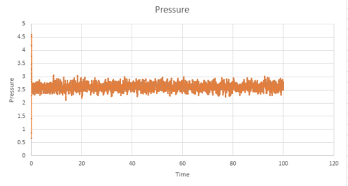
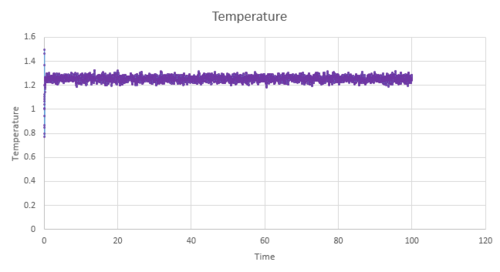
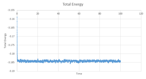
Figure 11-13 present the pressure, temperature and total energy for the simulation values run at a timestep value of 0.001. This system equilibrates very quickly approximately at 0.5, as the three factors of pressure, temperature and total energy have a constant value and naturally fluctuate around this average value. It can be concluded that the equilibration time would be independent of the timesteps; however, the smaller the timesteps are, a greater level of detail is able to captured by this system. Therefore, the total average energy would be independent of the number of timesteps as long as the values used in the average are taken from when the system is at thermodynamic equilibrium.

molecule1
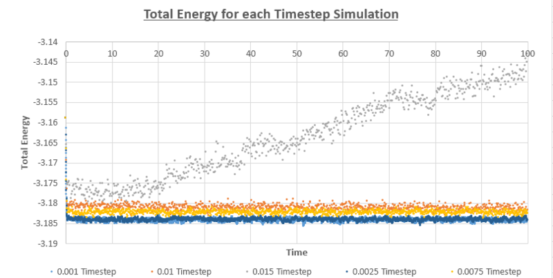
Figure 14: Total Energy against time for different timestep values in simulation

TASK: Of the five timesteps that you used, which is the largest to give acceptable results? Which one of the five is a particularly bad choice? Why?

The 0.0015 timestep would not be suitable as the total energy is significantly increasing for the system with time and thus does not reach thermodynamic equilibrium. For the 0.01 and the 0.0075 timesteps, it appears that the total energy is still decreasing with time. The 0.001 and 0.0025 timesteps have the same average energy. Out of these two timesteps that have reached thermal equilibrium, it would be most ideal to use the larger, 0.0025 timestep as the system would be observed over a larger period of time.

Task 4 - Running simulations under specific conditions

Solve these equations to determine $\gamma$.

$\frac{1}{2}\sum _i{m}_i{v}_i^2=\frac{3}{2}N{k}_{B}T$

$\frac{1}{2}\sum _i{m}_i{\gamma }^2{v}_i^2=\frac{3}{2}N{k}_B\tau$

Using the equations above, the following equation can be obtained:

$\frac{1}{{\gamma }^2}=\frac{T}{\tau }$

${\gamma }^2=\frac{\tau }{T}$

$\gamma =\pm \sqrt{\frac{\tau }{T}}$

TASK: Use the manual page to find out the importance of the three numbers 100 1000 100000. How often will values of the temperature, etc., be sampled for the average? How many measurements contribute to the average? Looking to the following line, how much time will you simulate?

The following line of code describes, the frequency and the number of timesteps that will be used to contribute to the average.

fix aves all ave/time 100 1000 100000 v_dens v_temp v_press v_dens2 v_temp2 v_press2

The code is organised into the following format:

fix aves all ave/time Nevery Nrepeat Nfreq.......

• Nevery = the gap between the timestep values that will be used to calculate the average

• Nrepeat = the number of data point that are used to calculate the average

• Nfreq = the calculation of averages every Nfreq timestep

Therefore, for the code above, the average will be calculated every 100,000 timesteps using 1000 data inputs that are spaced every 100 timesteps. As the timestep was defined to be 0.025, the total time the system is simulated for:

$$\begin{gathered} Total \\ time=100,000\times 0.0025=250 \\ time \\ units \end{gathered}$$

Plotting the Equations of State

The following values set the NpT ensemble conditions, with constant temperatures and pressures simulated using the LAMMPS platform. This resulted in 10 simulations:

Temperature: 1.5, 1.6, 1.7, 1.8, 1.9

Pressure: 2.50, 2.60

Timestep: 0.0025 (as previously obtained for Task 2)

molecule1	molecule1
Figure 15: The density varying with temperature + ideal gas values	Figure 16: The density varying with temperature (experimental values with addition of error bars)

It was found that with a increase in the temperature, the density decreased; ie expansion of the material. The observed graphical shape was consistent with a inverse relationship between these two variables. When the system is heated, the volume occupied would increase, due to the atoms taking up more space due to the increasing degrees of freedom and the total mass remaining the same. . The increase in pressure would be equivalent to increasing the density of the material (through Boyle's Law) and therefore the increase in the pressure would cause a transformation of the curve to higher density values. Superimposing the theoretical ideal gas curve to the experimental data, it was observed that the ideal gas density values are substantially higher that the computed values.

The difference in the values is due to the assumption made in the ideal gas model; the particles having no interactions between the other particles in the system and the particles having no volume (ie point particles). In this theoretical setting it would be possible to have the particles on top of one another and at higher densities. In this experiment, the repulsive component of the Lennard-Jones Potential would prevent this from occurring. The ideal gas only agrees well with experimental data in the low density systems, where the number of interactions are minimal. It is observed in Figures 15, that the difference in Lennard-Jones Potential and the theoretical ideal gas system increases with pressure due to the same argument relating to the interactions and density assumptions.

Task 5 - Calculating heat capacities using statistical physics

The simulations were calculated using the following conditions:

Density: 0.2, 0.8

Temperature: 2.0, 2.2, 2.4, 2.6, 2.8

Number of atoms 3375

The volume of the system was found by the following equation: $$\begin{gathered} V=\frac{Number \\ of \\ atoms}{Density} \end{gathered}$$

molecule1
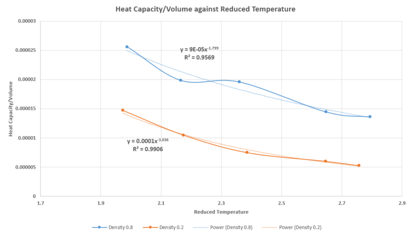
Figure 17: A plot of the Heat Capacity/Volume with respect to temperature

The heat capacity is the energy required to raise the temperature of one unit mass of the substance, by one degree K.

• The trendline for the Heat Capacity was used, as it provided the best match to the data points ie $greater{R}^{2}value$.

• As the temperature of the system increased, the heat capacity of the system decreased. This occurs because the increase in temperature results in the amount of energy that the system absorbs is decreased from the increase of internal energy of the system. This is analogous to the two level system in statistical thermodynamics.

• The increase in density would lead to a increase in the value of the heat capacity. As the density is defined as the mass per unit volume, the increase in density is equivalent to an increase of the mass packed into a unit cell of constant volume in the system. Furthermore, the increase in density means there is a greater number of the microstates that the system can occupy as the number of degrees of freedom of the unit cell increases - thus leading to an increase in the energy required to raise the temperature of a unit mass of the system, by 1K.

Comparing the experimental values to the ideal gas system:

$U=\frac{3}{2}nRT$ as an ideal gas system has 3 translational degrees of freedom. This is consistent with the equipartition theorem which states that the each degree of freedom in system would contribute $U=\frac{1}{2}nRT$

to the total internal energy of the system.

For a 1 mole system:

$U=\frac{3}{2}RT$

As $C_{\text{V}}={\left(\frac{\partial U}{\partial T}\right)}_{\text{V}}$

$C_{\text{V}}={\left(\frac{\partial \frac{3}{2}RT}{\partial T}\right)}_{\text{V}}$

$C_{\text{V}}=\frac{3}{2}R$ ie CONSTANT VALUE

Under the ideal gas law, the Heat Capacity is constant for the system. It is independent of the temperature.

Input Code for Calculation of Heat Capacity

 
### DEFINE SIMULATION BOX GEOMETRY ###
variable density equal 0.2

lattice sc ${density}
region box block 0 15 0 15 0 15
create_box 1 box
create_atoms 1 box

### DEFINE PHYSICAL PROPERTIES OF ATOMS ###
mass 1 1.0
pair_style lj/cut/opt 3.0
pair_coeff 1 1 1.0 1.0
neighbor 2.0 bin

### SPECIFY THE REQUIRED THERMODYNAMIC STATE ###
variable T equal 2.0
variable p equal 2.6
variable timestep equal 0.0025

### ASSIGN ATOMIC VELOCITIES ###
velocity all create ${T} 12345 dist gaussian rot yes mom yes

### SPECIFY ENSEMBLE ###
timestep ${timestep}
fix nve all nve

### THERMODYNAMIC OUTPUT CONTROL ###
thermo_style custom time etotal temp press
thermo 10

### RECORD TRAJECTORY ###
dump traj all custom 1000 output-1 id x y z

### SPECIFY TIMESTEP ###

### RUN SIMULATION TO MELT CRYSTAL ###
run 10000
unfix nve
reset_timestep 0

### BRING SYSTEM TO REQUIRED STATE ###
variable tdamp equal ${timestep}*100
fix nvt all nvt temp ${T} ${T} ${tdamp}
run 10000
unfix nvt
fix nve all nve
reset_timestep 0

### MEASURE SYSTEM STATE ###
thermo_style custom step etotal temp atoms density
variable n2 equal atoms*atoms
variable energy equal etotal
variable energy2 equal etotal*etotal
variable temp equal temp
variable temp2 equal temp*temp
variable Number equal atoms
variable dens equal density
variable dens2 equal density*density
fix aves all ave/time 100 1000 100000 v_energy v_energy2 v_temp v_temp2 v_dens
run 100000

variable CV equal (((f_aves[2]-f_aves[1]*f_aves[1])/(f_aves[4]))*${n2})
variable avetemp equal f_aves[3]
variable avedens equal f_aves[1]

print "Temperature: ${avetemp}"
print "Heat Capacity: ${CV}"
print "Atoms: ${Number}
print "Density: ${avedens}"

Radial distribution function - Task 6

molecule1	molecule1
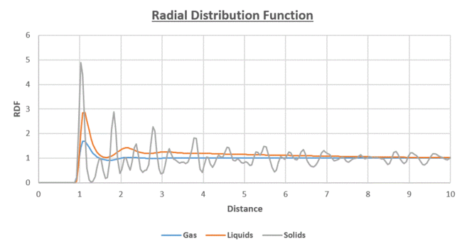
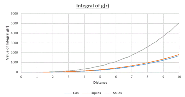
Figure 18: Radial Distribution Function for the Lennard-Jones Potential at the different states of matter	Figure 19: Integral of the radial distribution function

• The radial distribution function describes the effective density of particles relative from a reference particle; it is equivalent to the probability of finding a particles at a distance r from the reference particle. The RDF is a effective method of assessing the order in the molecule systems.

• The integral of g(r) ie the area under the RDF curves, is equal to the density of the particles.

Figure 18 illustrates the radial distribution function for the different states of the system at a given distance from a reference atom; in the solid, liquid and gas phases.

• The number of peaks for each state indicates the degree of ordering. ie the solid has the highest degree of ordering
• At $$\begin{gathered} r \\ =0 \end{gathered}$$ the $$\begin{gathered} RDF \\ =0 \end{gathered}$$, for all the states.
• At short distances of r, the RDF=0. Below this distance, the atoms would be overlapping.
• For the liquid and gaseous states, the 1st peak corresponds to the minima of the Lennard-Jones Potential at $$\begin{gathered} r \\ =1.125 \end{gathered}$$
• As the distance r increases from the reference particle, the solid, liquid and gas states all tend towards a constant average effective density of 1 (1 is the bulk density of the system).

The solid is found to have a greater number of peaks and larger amplitudes of fluctuation, than the liquid and gas states. This is due to the fixed and highly ordered nature of the particles in the lattice structure, with short and long range ordering present due to the peaks present at short and long range. There is minimal degrees of freedom as the particles are in fixed lattice positions. In addition, the larger amplitude of the peaks which is especially clear from the peak closest to the reference particles, indicates a greater packing density than the liquid and gas systems; a larger number of particles are packed into a smaller distance (volume in 3-D). The oscillating nature of the RDF is analogous to a trigonometric function. This behaviour is observed due to the greater density of particles at certain distances from the reference particle and absent or minimal at the other distances.

For example: In the solid state system with $$\begin{gathered} Density \\ =1.2 \end{gathered}$$

In a fcc lattice with 4 atoms, this corresponds to a $$\begin{gathered} Side \\ length \\ a \\ (Lattice \\ Parameter) \\ =1.493801582... \end{gathered}$$

Nearest neighbours in a fcc lattice are at $$\begin{gathered} \frac{\sqrt{2}}{2}a, \\ a \\ and\frac{\sqrt{6}}{2}a \end{gathered}$$. Where a is the lattice parameter for the system. It would be expected that the first 3 peaks in Figure 18, correspond to the theoretical values of $$\begin{gathered} r \\ =1.06 \\ (3sf) \end{gathered}$$,$$\begin{gathered} r \\ =1.49 \\ (3sf) \end{gathered}$$ and $$\begin{gathered} r \\ =1.83 \\ (3sf) \end{gathered}$$. These predictions are in agreement with the experimental data in Figure 18, with maxima peaks found at $$\begin{gathered} r \\ =1.025 \end{gathered}$$, $$\begin{gathered} r \\ =1.475 \end{gathered}$$ and $$\begin{gathered} r \\ =1.825 \end{gathered}$$.

It was found from Figure 19, the $$\begin{gathered} Co-ordination \\ number \\ for \\ reference \\ atom(r⩽1.825)=32.72840345\approx 33 \end{gathered}$$ for the solid state. This is equivalent to the area of the first three peaks for the solid state in figure 18.

For the liquid system, there were fewer peaks found in figure 18. This is due to the increase in the number of degrees of freedom, with 3 translation vectors. The liquid reaches an equilibrium density closer to the reference system, than for the solid as there is a short range order. In additional, there is a Lennard-Jones interaction present which leads to the formation of a local minima and some degree of short range ordering, as seen by the multiple peaks close to the reference atom. For the gas state, there is one obvious peak in system and the distance for the maximum effective density of particles is approximately the same as the liquid system (figure 19); the peak is of lower value than the liquid maxima. This is likely due to the random Brownian motion of the particles and the ability of the molecules in this gaseous state (to an extent the liquid phase) to freely move in the box. The lack of peaks present indicates there is no ordering present in the gaseous state. Furthermore, the peak present for the gaseous states is much broader than the solid or liquid states. This is due to the thermal motion of the atoms, which occurs at higher temperatures.

Dynamical properties and the diffusion coefficient - Task 7

TASK: make a plot for each of your simulations (solid, liquid, and gas), showing the mean squared displacement (the "total" MSD) as a function of timestep. Are these as you would expect? Estimate $D$ in each case. Be careful with the units! Repeat this procedure for the MSD data that you were given from the one million atom simulations.

The diffusion co-efficient was able to be established, using the relationship to the mean squared displacement (as seen below). Please find the D-coefficient values in the table below:

$D=\frac{1}{6}\frac{\partial ⟨r^2\left(t\right)⟩}{\partial t}$

molecule1	molecule1
Figure 20: The plot of the mean squared displacement against timesteps	Figure 21: The close up of the non-linear region of the plotting in the mean squared displacement against timesteps

molecule1
Figure 22: The plot of the mean squared displacement against timesteps for a million atoms

TASK: In the theoretical section at the beginning, the equation for the evolution of the position of a 1D harmonic oscillator as a function of time was given. Using this, evaluate the normalised velocity autocorrelation function for a 1D harmonic oscillator (it is analytic!):

Derivation:

$C\left(\tau \right)=\frac{\underset{-\mathrm{\infty }}{\overset{\mathrm{\infty }}{\int }}v\left(t\right)v(t+\tau )\mathrm{d}t}{\underset{-\mathrm{\infty }}{\overset{\mathrm{\infty }}{\int }}{v}^2\left(t\right)\mathrm{d}t}$

As $x\left(t\right)=A\cos (\omega t+\varphi )$ is the displacement over time for the system.

$\frac{\partial \left(x\left(t\right)\right)}{\partial t}=v\left(t\right)$ is the velocity over time for the system

$v\left(t\right)=-\omega A\sin (\omega t+\varphi )$ is the velocity of the 1-D harmonic oscillator

$C\left(\tau \right)=\frac{\underset{-\mathrm{\infty }}{\overset{\mathrm{\infty }}{\int }}-\omega A\sin (\omega t+\varphi )v(t+\tau )\mathrm{d}t}{\underset{-\mathrm{\infty }}{\overset{\mathrm{\infty }}{\int }}{\omega }^2{A}^2{\sin }^2(\omega t+\varphi )\mathrm{d}t}$

$C\left(\tau \right)=\frac{\underset{-\mathrm{\infty }}{\overset{\mathrm{\infty }}{\int }}-\omega A\sin (\omega t+\varphi )\times -\omega A\sin (\omega (t+\tau )+\varphi )\mathrm{d}t}{\underset{-\mathrm{\infty }}{\overset{\mathrm{\infty }}{\int }}{\omega }^2{A}^2{\sin }^2(\omega t+\varphi )\mathrm{d}t}$

$C\left(\tau \right)=\frac{\underset{-\mathrm{\infty }}{\overset{\mathrm{\infty }}{\int }}\omega A\sin (\omega t+\varphi )\times \omega A\sin (\omega t+\omega \tau +\varphi )\mathrm{d}t}{\underset{-\mathrm{\infty }}{\overset{\mathrm{\infty }}{\int }}{\omega }^2{A}^2{\sin }^2(\omega t+\varphi )\mathrm{d}t}$

Furthermore, $\sin (A+B)=\sin \left(A\right)\cos \left(B\right)+\sin \left(A\right)\cos \left(B\right)$

Let $(\omega t+\varphi )=A$ and $\omega \tau =B$

$\sin (t+\tau )=\sin (\omega t+\varphi )\cos \left(\omega \tau \right)+\sin \left(\omega \tau \right)\cos (\omega t+\varphi )$

$C\left(\tau \right)=\frac{{\omega }^2{A}^2\underset{-\mathrm{\infty }}{\overset{\mathrm{\infty }}{\int }}\sin (\omega t+\varphi )\times \sin (\omega (t+\tau )+\varphi )\mathrm{d}t}{{\omega }^2{A}^2\underset{-\mathrm{\infty }}{\overset{\mathrm{\infty }}{\int }}{\sin }^2(\omega t+\varphi )\mathrm{d}t}$

$C\left(\tau \right)=\frac{\underset{-\mathrm{\infty }}{\overset{\mathrm{\infty }}{\int }}\sin (\omega t+\varphi )\times [\sin (\omega t+\varphi )\cos \left(\omega \tau \right)+\sin \left(\omega \tau \right)\cos (\omega t+\varphi )]\mathrm{d}t}{\underset{-\mathrm{\infty }}{\overset{\mathrm{\infty }}{\int }}{\sin }^2(\omega t+\varphi )\mathrm{d}t}$

$C\left(\tau \right)=\frac{\underset{-\mathrm{\infty }}{\overset{\mathrm{\infty }}{\int }}\sin (\omega t+\varphi )\times \sin (\omega t+\varphi )\cos \left(\omega \tau \right)\mathrm{d}t+\underset{-\mathrm{\infty }}{\overset{\mathrm{\infty }}{\int }}\sin (\omega t+\varphi )\sin \left(\omega \tau \right)\cos (\omega t+\varphi )\mathrm{d}t}{\underset{-\mathrm{\infty }}{\overset{\mathrm{\infty }}{\int }}{\sin }^2(\omega t+\varphi )\mathrm{d}t}$

As we can assume the values of $\cos \left(\omega \tau \right)=Constan{t}_1$ and $\sin \left(\omega \tau \right)=Constan{t}_2$

$C\left(\tau \right)=\frac{\cos \left(\omega \tau \right)\underset{-\mathrm{\infty }}{\overset{\mathrm{\infty }}{\int }}{\sin }^{}(\omega t+\varphi )\mathrm{d}t+\sin \left(\omega \tau \right)\underset{-\mathrm{\infty }}{\overset{\mathrm{\infty }}{\int }}\sin (\omega t+\varphi )\cos (\omega t+\varphi )\mathrm{d}t}{\underset{-\mathrm{\infty }}{\overset{\mathrm{\infty }}{\int }}{\sin }^2(\omega t+\varphi )\mathrm{d}t}$

$C\left(\tau \right)=\cos \left(\omega \tau \right)+\frac{\sin \left(\omega \tau \right)\underset{-\mathrm{\infty }}{\overset{\mathrm{\infty }}{\int }}\sin (\omega t+\varphi )\cos (\omega t+\varphi )\mathrm{d}t}{\underset{-\mathrm{\infty }}{\overset{\mathrm{\infty }}{\int }}{\sin }^2(\omega t+\varphi )\mathrm{d}t}$

As $\sin \left(\omega \tau \right)\underset{-\mathrm{\infty }}{\overset{\mathrm{\infty }}{\int }}\sin (\omega t+\varphi )\cos (\omega t+\varphi )\mathrm{d}t\to 0$ due to the the property of $$\begin{gathered} Odd \\ function\times \\ Even \\ function \\ = \\ Odd \\ Function \end{gathered}$$

$\therefore \underset{-\mathrm{\infty }}{\overset{\mathrm{\infty }}{\int }}\sin (\omega t+\varphi )\cos (\omega t+\varphi )\mathrm{d}t=0$

SOLUTION:$\therefore C\left(\tau \right)=\cos \left(\omega \tau \right)$

Diffusion Co-efficient (unit area/time) to 3sf	MSD	MSD (Million atoms)	VCAF	VCAF (Million atoms)
Gas	3.21	2.44	3.38	3.27
Liquid	0.0689	0.0698	0.0697	0.0901
Solid	5.00E-6	3.33E-06	1.89E-4	4.60E-5

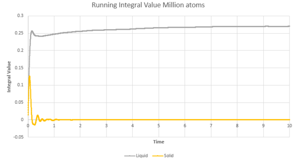
The trend of the diffusion co-efficients are in agreement with what would theoretically would be expected. The increase in the number of atoms did not produce a significant change in the value of D. The values were similar to the previously calculated values in the original VCAF and MSD. The largest source of the error in the VCAF would originate from the use of the trapeizum rule that approximates the area under the curve and the timestep value used. The calculation of the absolute integral would increase the reliability of the result, while decreasing the timestep value would increase the number data points of the curve.

As seen in Figure 20-22, the mean squared displacement of the particles initially follows a parabolic curve behaviour and then stabilizes to a linear relationship. The vapour presents the initial greatest curvature, followed by the liquid and gas. This due to a molecule at very small time values travelling in a straight trajectory until it collides with another molecule. Before the respective molecule undergoes its first collision, the velocity of the molecule would be constant, and therefore the $MSD\propto t^2$(parabolic behaviour). The point at which the collisions start to occur with the other molecule/the MSD becomes a $MSD\propto t$ relationship occurs at time values t(solid)<t(liquid)<t(gas) for the respective states. This is due to the gas molecules on average being further apart from one another. They have to travel a greater distance to interaction and collide with other molecules. On the other hand, in the solid state the atoms are in fixed positions with co-ordination to the surrounding atoms, leading to very fast stabilisation to a linear MSD behavior.

The D(Solid) < D(Liquid) < D(Vapour). For the solid state system, the values of the diffusion coefficient are very low and thus indicates the time for a particle to diffuse through the system would be large. This would be due to atoms in the lattice system being in fixed positions. In the liquid state, there are a greater degrees of freedom, relative to the solid state ie translational degrees of freedom, which contributes to the larger diffusion coefficient. However, there are still interactions between the particles from the short range. The vapour state has the greatest value of the diffusion co-efficient due to the greatest degree of freedom for the system and ability to diffuse through the system at a faster rate due to only very weak forces interacting.

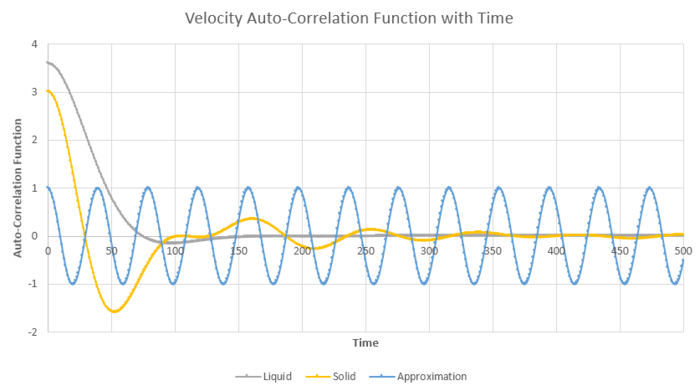
The behaviour in figure 23 can be explained by the interactions of the particles for the different states of matter. If the particles of the system did not interact with one another, then the velocity of the particles would remain constant at their starting velocities. However, due to the forces of interaction from the neighboring particles, the velocity of a reference particle changes over time.

The liquid does not have fixed lattice positions and a long range interactions. Figure 23 illustrates the diffusive, brownian motion of the particles in the liquid system and the collisions with the other neighboring particles, causing a sharp dampened oscillation at a low value of t. For the solid, the atoms are in fixed positions of the lattice structure and are packed together in high densities, as seen from the integral of g(r) in task 6. As there would be multiple forces and interactions for a given atom, the atom would seek to find the lowest minima energy point on its potential energy surface. This leads to the oscillation in the velocity well, found in figure 23 for the solid state. The perbutations and collisions with the surrounding atoms, would dampen the oscillations of the atom and decorrelate the velocity over time. The diffusive behaviour would mean that over time the energy is transferred throughout the lattice structure to increase the overall entropy of the system. The velocity of the reference atom would tend close to 0 for t infinite.

The harmonic oscillator provides a good approximation for locating the values of t, which give the minimum values in the solid and the liquid states. There are no collisions that occur in the harmonic oscillator and therefore the force constant of the oscillations will remain constant in the opposite direction of displacement. This produces the non-decaying oscillating behaviour as seen in figure 23.

molecule1
Figure 23: The plot of the velocity auto correlation function for 500 timesteps in the liquid and solid states

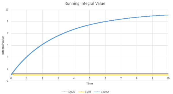
The greatest error is associated with the gaseous state, due to the largest curvature for the running integral in figure 24 & 25 for both the million atoms and the original simulations. This is due to the trapezium rule underestimating the value of the integral. Using smaller timesteps would help to reduce this error by producing a better trapezium approximation to the curve and thus a more accurate value of the integral. The solid state would have the lowest associated error due to the stable linear nature of the curve, leading to approximations using the MSD and the VCAF via the trapezium rule being possible and accurate.

molecule1	molecule1
Figure 24: The VCAF running integral approximated by the trapezium rule	Figure 25: The VCAF running integral approximated by the trapezium rule for the solid and liquid phase

molecule1	molecule1
Figure 26: The VCAF running integral approximated by the trapezium rule for the million atoms	Figure 27: The VCAF running integral approximated by the trapezium rule for the solid and liquid phase million atoms simulations