Rep:Mod:lierke

Introduction to molecular dynamics simulation

Theory Behind Molecular Dynamics Simulations

Molecular dynamics studies the behaviour of atoms as a function of time. It is a technique which is often applied to bioinformatics. Using ‘MD,’ information about fluctuations in conformations of proteins, nucleic acids etc. can be obtained. It is also a vital tool in determining how ion channels operate. Due to the lack in computational power to simulate the entire universe, molecular dynamics makes use of several approximations to generate an accurate and better understanding of the thermodynamics, and dynamics of molecular systems. Molecular dynamics is a useful tool, on the assumption that the number of atoms in the system that is being studied, remains constant. If this is not the case, molecular dynamics is not as useful, and other methods such as Monte Carlo simulations must be employed. Understanding the input and output of a molecular dynamics simulation is essential to understanding the value of the results obtained. Statistical mechanics is a tool that allows the microscopic properties (positions, and velocities of atoms) obtained through MD to be converted into more useful properties which are of a macroscopic nature including the pressure, temperature, energy, heat capacity etc. With Molecular dynamics, the motion of the atoms is studied, which can be used to solve the equations which allow the determination of thermodynamic and kinetic properties. Up to now, molecular dynamics has been described in a simplified way, however to determine accurate results of complex systems, several modifications need to be made to generate an accurate simulation.

Interaction Potentials

A simulation could be run, assuming that all the atoms in a given space, which we will assume to be a box, do not interact. This however would be a very crude approximation, because in reality we know that all atoms in this box have a force acting on them. This force is a result of atoms interacting with one another. The set of rules that define the nature and strength of these interactions is referred to as the interaction potential. It is for this particular reason that force fields need to be very accurate for the system on which the simulation is being run. In reality all atoms interact with one another, but even in small systems with several thousands of atoms this would be very expensive to compute. It is therefore necessary that simplifications are applied. One of such simplifications is the use of a cut off distance, which assumes that beyond a certain distance, atoms do no interact (this is often referred to as a screening effect). The general equation for the overall interatomic potential can be written as follows:

|

Where each of the different components is defined as:

V_bonded = Covalent or ionic bonds

V_non-bonded = Lennard Jones or coulombic

V_restraints = E.g pinning of hydrogen atoms

V_field = The effects on the interatomic potential from e.g the solvent, magnetic field, or electric field.

Bonding

Each of these separate contributions are evaluated with mathematical equations. The Vbonded contribution of the interatomic potential is derived from simple mathematical formulae. While simple, these formulae are relatively accurate. The need for these formulae to be simple stems from the fact that forces are updated every step. If the formulae used to determine Vbonded were too complex, the simulation would not run properly.

Non-Bonding

All neighbours for an atom are computed, and the interactions with the atom that is observed are added together. In ideal circumstances, a pair wise additive approach is used, because it simplifies the calculations, and avoids more complex calculations which incorporate multi-body effects. However in certain simulations which study more complex systems such as metals, we cannot make use of pairwise interactions, because atoms are too close in proximity. In these simulations, multibodies are used. In the case of the Lennard Jones potential, a pure pairwise additive is assumed. Calculations based on this assumption are a lot quicker than alternatives such as MEAM, or EAM.

EAM vs MEAM

EAM and MEAM are essential for more complex systems. MEAM is essentially a more complex version of EAM, where directionality, radial, and angular contributions are taken into account. These added features in MEAM, allow simulations to be run on complex crystals, such as diamond.

Verlet Algorithm

It turns out that treating atoms like classical particles is a good approximation. The different parameters used to described the properties of these classical particles are outlined below.

F_i = Force acting on atom i

M_i = Mass of atom i

A_i = Acceleration of atom i

V_i = Velocity of atom i

X_i = position of atom i

It turns out that Newtonian formulae can be used to accurately describe what is going on in molecular dynamics.

|

In systems of few atoms (e.g 10), it would not be difficult to generate these properties. However most systems, such as studying the behaviour of a liquid is far too complex to solve without using computers. It is for this reason that molecular dynamics is useful. Treating the positions, velocities etc. as continuous would require a large amount of computer power. Instead, timesteps are used. The algorithm of choice to determine these Newtonian properties is the Verlet algorithm. The Verlet algorithm is the algorithm of choice, because although simple in nature, it does a very good job at preserving the energy of the system that is being studied. While we won’t make use of any real units of time in our simulations (we will use reduced units), in terms of getting an idea on which timescale these types of simulations are run, best timesteps for most force fields are usually on the order of 1-2 femtoseconds.

Limitations to the Verlet theorem include the fact that velocities are not calculated. Without the velocities, essential properties such as the energy of the system cannot be determined. It is for this reason that modifications to the Verlet theorem were made, which led to the Velocity Verlet theorem. On the assumption that the acceleration of an atom is independent on its velocity, and only dependent on its position, we can generate the Velocity Verlet algorithm. This algorithm allows us to calculate the atomic velocities explicitly.

Using the Velocity Verlet equation, it is essential that we know the initial positions/velocities of all the atoms in the system on which the simulation is being performed.

|

Effects of changing the mass

Increasing the Mass

|

Explanation:

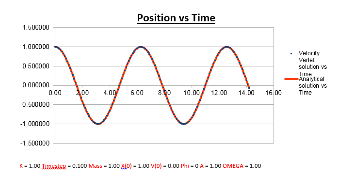
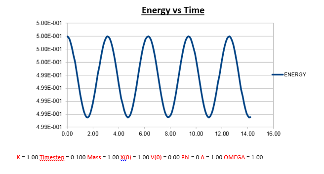
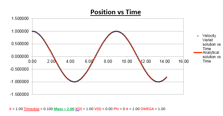
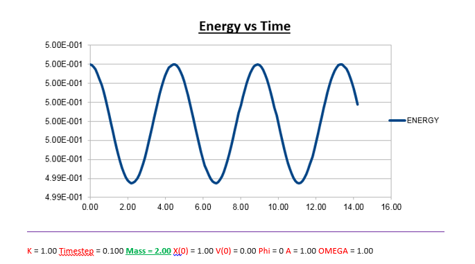
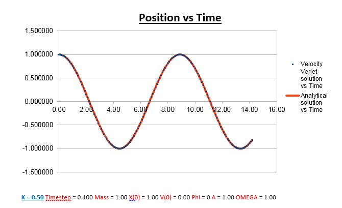
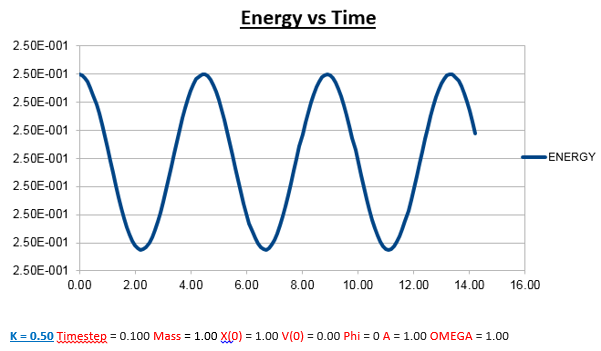
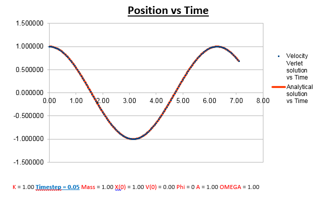
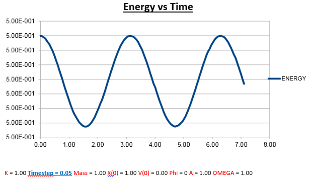
As can be seen from the graphs illustrated above, the frequency decreases in both the position vs time and energy vs time graphs, as the mass is increased. Knowing that the Velocity Verlet data accurately corresponds to that of the classical harmonic oscillator, we can find a plausible explanation by analysing how incresasing the mass would influence the frequency of a classical harmonic oscillator.

|

Where ω = frequency, k = force constant and µ = reduced mass.

We can predict that an increase in the mass and thus an increase in the reduced mass (if m = 2, µ = 1, compared to if m = 1, µ = 0.5) will lead to an overall lower value for the frequency. Similarly we can decrease the mass compared to its original value (1.00), and an increase in overall frequency in both energy vs time (how quick the energy fluctuates), and in the position vs time graphs should be observed. This is illustrated below.

Decreasing the mass

|

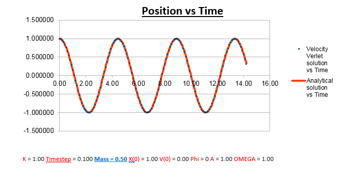
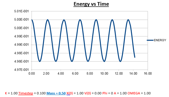
Explanation: Instead of increasing the mass like last time, the mass has now been decreased to 0.5, resulting in a reduced mass of 0.25. Using the formula for the frequency of a classic harmonic oscillator described earlier, we can predict that the frequency should increase as the mass is decreased, which matches what we observe in both the position vs time, and energy vs time graphs.

Increasing the Force Constant

Effects of changing the force constant

|

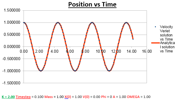
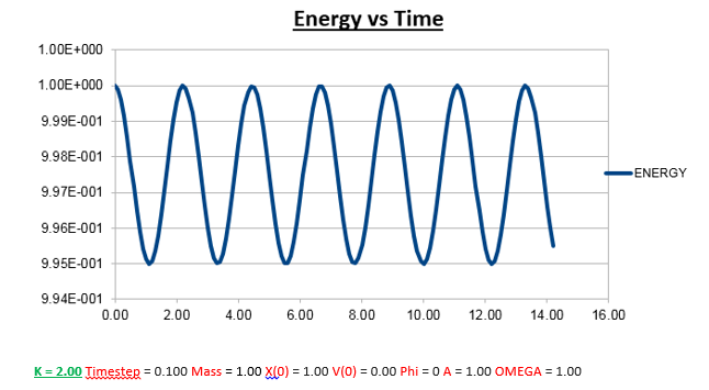
Explanation: In contrast to the trend observed as the mass was varied, the frequency in both the position vs time, and energy vs time graphs increases as the force constant is increased (again using the classical harmonic oscillator formula for determining the frequency).

Decreasing The Force Constant

|

Explanation: Analogous to the explanation for when the force constant was increased, decreasing the force constant results in the opposite trend (a decrease in frequency).

Increasing the Time-Step

|

Decreasing The Time-Step

|

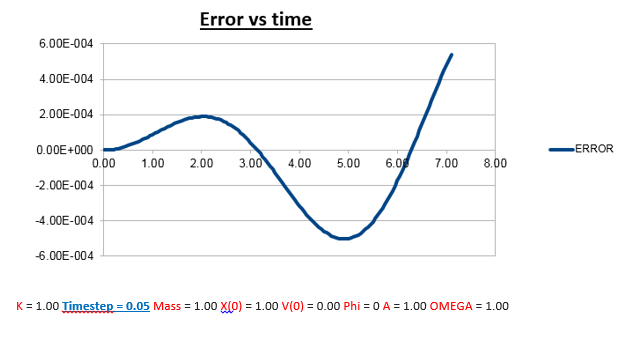
TASK: Why do you think the error in the position changes with time in the way that it does?

|

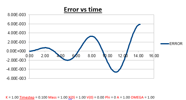
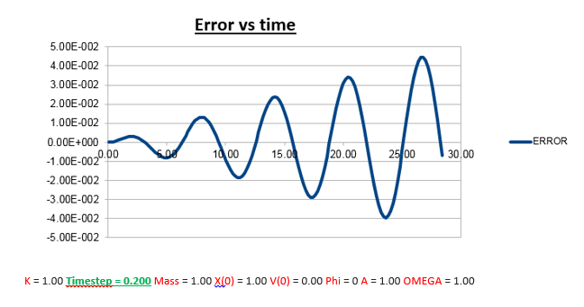
Explanation: There are several noticeable things about this error vs time graph.

1)Error oscillates as a function of time, but as time progresses, the oscillations are also observed to have a greater amplitude.

         a) This can be described approximately by the multiplication of a wave by an envelope function (complex wave).

2)The reason the error oscillates over time is because the change in position also has a change in error attached to it. The larger the velocity (the faster the position changes), the less good the taylor approximation holds, which is what we used to derive the Velocity-Verlet algorithm.

Increasing the mass

|

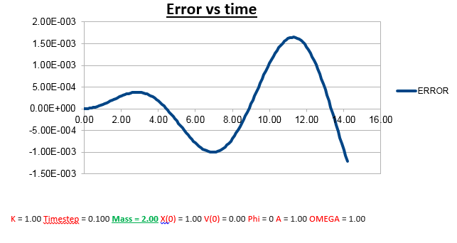
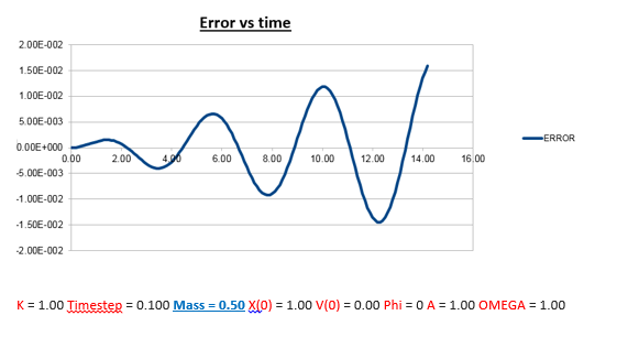
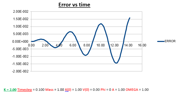
Explanation: Comparing the error vs time graph of the conditions we used to run the simulation, and the error vs time graph when we doubled to mass (2.00 vs 1.00), we notice less frequent oscillations. To explain this, we need to understand the nature of how the error was determined. As instructed by the script, the error is defined as the difference between the analytical and Velocity -Verlet solution for x(t). Therefore we expect an increase in ‘error’ when the error in the Velocity-Verlet solution becomes bigger. Therefore to understand why and when the error gets bigger, we can also be determine where/when the Velocity-Verlet algorithm starts to break down. Knowing (as previously described) that the Velocity-Verlet algorithm is based on a Taylor expansion, for the Taylor expansion to be accurate, we need the timesteps to be small, so that the change in position as a function of time is relatively small. However, knowing that the velocity also varies as a function of time, we know that the error must also vary as a function of time. The faster an atom is moving, the greater its displacement for the same time step. So the greater the velocity, the greater the error, which explains the change in the frequency of oscillation.

Why does the amplitude of the oscillation in error increase as a function of time?

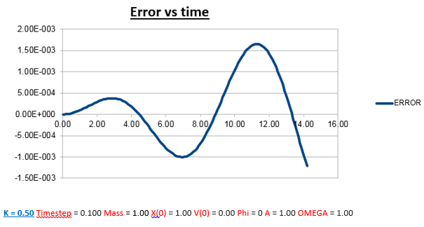
The error gets larger over time, because it accumulates. At every time-step there is a given error, which varies, as a function of time, but due the fact that there always a finite error at every time-step, it’s safe to assume that the overall error (which is the sum of all the errors at each time-step) will increase, which is what we observe.

Decreasing the mass

|

Increasing the Force Constant

|

Decreasing the Force Constant

|

Increasing the Timestep

|

Decreasing the Timestep

|

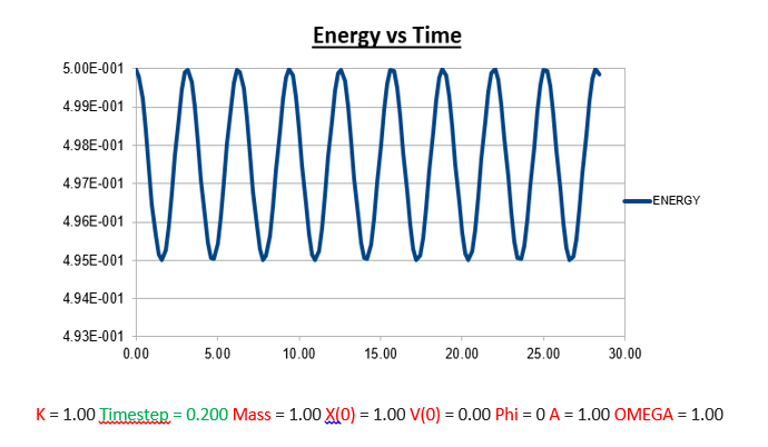
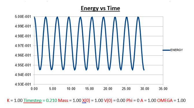
Task: What sort of a timestep do you need to use to ensure that the total energy does not change by more than 1% over the course of your "simulation"?

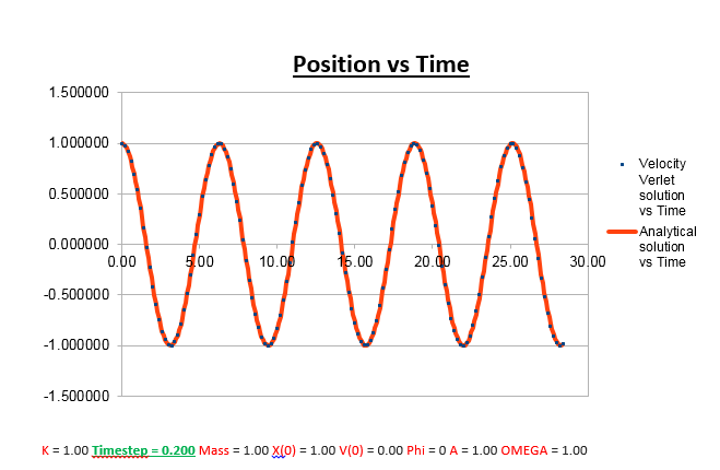
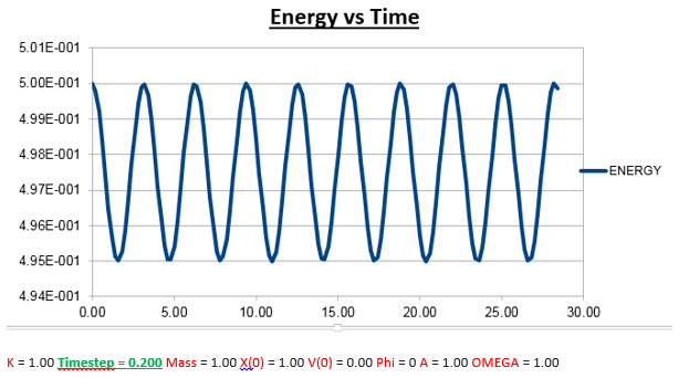
From the analysis above, where we manipulated the timestep value, we came to the conclusion that the the change in total energy becomes larger as the timestep is increased. Knowing that 1% of the starting energy (0.5) is equal to 0.01. The energy vs time graph can thus never reach a value lower than 0.495. As the timestep value is increased to 0.2, we can see that the value oscillates from a maximum of 0.5 to a minimum of 0.495. Below we will illustrate the energy vs time graph with a timestep value of 0.2 as well as the same graph with a timestep which exceeds this value (0.21), and thus exceeding the allowed value of the error (more than 1%).

|

Task: Why do you think it is important to monitor the total energy of a physical system when modelling its behaviour numerically?

The total energy is a very useful property of a system to observe. Knowing that the law of conservation of energy must be obeyed at all times, we know that any change in total energy would lead to inaccurate results directly drawn from the simulation. An increase/decrease in energy is therefore a strong indication that the code written for the simulation is incomplete to obtain the desired simulation. For example if a simulation is run, and the energy is seen to increase as a function of time, we could try and add a heat sink, run the simulation again, and check whether an increase in energy is still observed, as the simulation progresses. If the energy is observed to stay constant, as the simulation is run, we can accurately conclude that the MD simulation ran is correct. However this does not necessarily mean we are simulating what we are looking for. Code runs exactly what you tell it to do, therefore if an input command is ambiguous, you might not be running the simulation you wanted to in the first place.

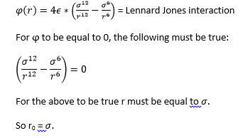
Task: Find the separation, r₀, at which the potential energy is zero.

|

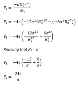
Task: What is the force at this separation?

|

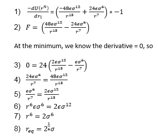
Task: Find the equilibrium separation, req.

|

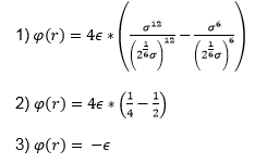
Task: Work out the well depth φ(r_eq)

Using the result we obtained in 8) we can now substitute this back into the equation for the Lennard-Jones interaction to obtain.

|

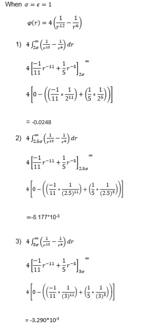
Task:Evaluate the integrals

|

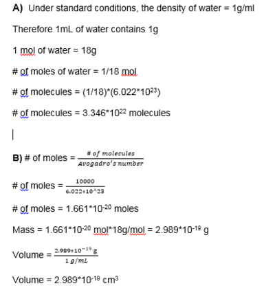
TASK: Estimate the number of water molecules in 1ml of water under standard conditions.

Task: Estimate the volume of 10000 water molecules under standard conditions.

|

TASK: Consider an atom at position (0.5, 0.5, 0.5) in a cubic simulation box which runs from (0. 0, 0) to (1, 1, 1). In a single timestep, it moves along the vector (0.7, 0.6, 0.2). At what point does it end up, after the periodic boundary conditions have been applied?

Imposing the boundary conditions, the atom moving from (0.5, 0.5, 0.5) along the vector (0.7, 0.6, 0.2) in a box which runs from (0. 0, 0) to (1, 1, 1), ends up at (0.2, 0.1, 0.7).

|

LJ cutoff = 3.2*(0.34nm) = 1.088 nm

Well depth = -Ɛ = ((120)*(1.38*10^-23)*(6.022*10²³))/(1000) = -0.997 kJ/mol

Reduced temperature = 1.5(120) (because Kb cancels) = 180K

Equilibration

Task: Why do you think giving atoms random starting coordinates causes problems in simulations? Think about what happens to the Lennard-Jones interaction between two atoms as they get very close together.

Totally random simulation can cause potential problems in simulation, because it doesn’t take into account the position coordinates of the other atoms, therefore there is a large probability that significant atoms will have overlapping interatomic potentials. This can significantly affect a simulation. Due to the nature of the Lennard Jones potential, taking on a high value as the interatomic distance is decreased beyond the equilibrium distance, we expect that these interatomic energies will be very high. If a simulation is run with just a few atoms, this might not be too much of a problem, but even in small systems of just a few 1000’s atoms, there can be several of these high interatomic energies. Calculations will as a result take a lot longer, and be of less significance when describing a real system. The large repulsive energy at these close interatomic distances will also cause the atoms to repel away from each other violently just beyond t = 0, as a result the beginning of the simulation will not give an accurate representation of a system at equilibrium! As a result, it might take longer for a system to reach an equilibrium.

Extra: Why do we often give atoms an initial value for the velocity when starting a simulation?

We do this because it is a bad idea to start with atoms being at rest (0K), as this would cause a so-called ‘thermal shock’ once we start the simulation.

A better approach is to draw the velocities from a standard Maxwell Boltzmann distribution function, at a given temperature.

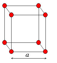
TASK: Satisfy yourself that this lattice spacing corresponds to a number density of lattice points of 0.8.

| source ²

|

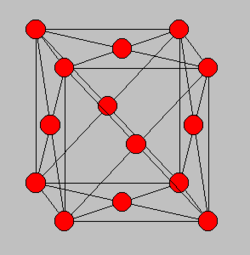
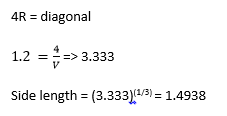
Task: Consider instead a face-centred cubic lattice with a lattice point number density of 1.2. What is the side length of the cubic unit cell?

| source ¹

|

TASK: Consider again the face-centred cubic lattice from the previous task. How many atoms would be created by the create_atoms command if you had defined that lattice instead?

Number of atoms per unit cell = (1/8)*8 + (1/2)*6 = 4

So in 1000 unit cells, we would expect a total of 4000 atoms to be created using the create_atoms command.

TASK: Using the LAMMPS manual, find the purpose of the following commands:

   mass 1 1.0
   pair_style lj/cut 3.0
   pair_coeff * * 1.0 1.0

Mass 1 1.0

Where the general formula states => Mass I Value

Where I = atom type

Value = the value of the mass of the atom type specified by I.

In the case of mass 1 1.0 the command is defining the mass of the atom type which is defined by the number, to have a mass of 1.0 Asterices are also often used in these types of command. If no number for I present in the command, and instead only an * is listed, it means that all atom types from 1 to N (where N is the number of atom types) have the same value for the mass which is consequently listed in the ‘value’ section of the command. In the case of a leading asterix, denoted *n, all atom types from 1 to n (inclusive) will have the mass defined by the value section of the command. If trailing asterix denoted n*, all atom types from n to N (inclusive), will have same value for the mass which is listed in the ‘value’ section of the command. A asterisk between two atom types, denoted m*n, means all atom types between m and n (inclusive) will have the same mass value denoted by the value selection of the command.

Pair_style lj/cut 3.0

The nature of this command is that it computes pairwise interactions. The pair potentials are defined between pairs of atoms, where a pair potential only exists if the atoms lie within the cut-off distance. Due to the fact that atoms are in continuous motion, the number of pair interactions changes as a function of time. In the case of the formula described above, the lj/cut stands for the cutoff lennard jones, with no coulombic interactions taken into account. In this case the arbitrarily defined distance is equal to 3.0.

pair_coeff * * 1.0 1.0

Has the general syntax:

pair_coeff I J args

Where I and J are atom types and args denotes the coefficients for one or more pairs of atom types.

The command allows the specification of the pairwise force field constants for a given amount of atom pair types.

TASK: Given that we are specifying Xi(0) and Vi(0), which integration algorithm are we going to use?

The velocity verlet algorithm, because this algorithm assumes that accelerations are independent of velocity, which allows us to calculate individual atomic velocities.

TASK: Look at the lines below.

### SPECIFY TIMESTEP ###
variable timestep equal 0.001
variable n_steps equal floor(100/${timestep})
variable n_steps equal floor(100/0.001)
timestep ${timestep}
timestep 0.001

### RUN SIMULATION ###
run ${n_steps}
run 100000

The second line (starting "variable timestep...") tells LAMMPS that if it encounters the text ${timestep} on a subsequent line, it should replace it by the value given. In this case, the value ${timestep} is always replaced by 0.001. In light of this, what do you think the purpose of these lines is? Why not just write:

timestep 0.001
run 100000

If we just wrote out:

timestep 0.001
run 100000

In that case each time you wanted to run that time step you would have to type out the value, whereas if you had defined it previously, all you would need to do is quote the variable you had defined it as, for instance ‘x’ which simplifies everything. This would be useful if the line of code was reoccurring, in case you wanted to change the nature of the variable, all you would need to do is change the way you defined the variable, and all the remaining code can be kept the same.

Tracking a Single Particle

|

Checking equilibration

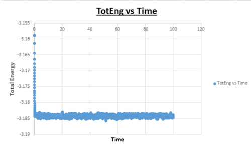
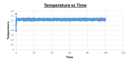
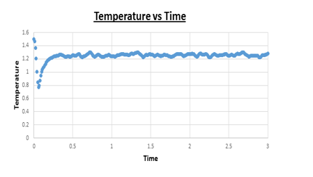
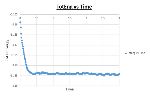
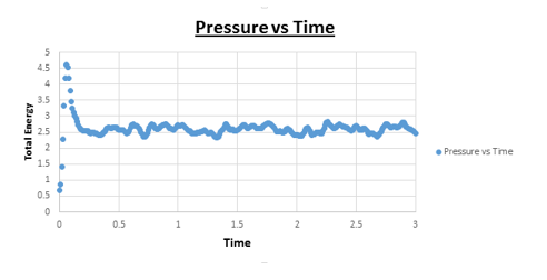
TASK: make plots of the energy, temperature, and pressure, against time for the 0.001 timestep experiment (attach a picture to your report).

|

Task: Does the simulation reach equilibrium?

Yes

Task: How long does this take?

~ t = 0.4 , we need to look at when the temperature, pressure, and total energy fluctuate about an average which remains constant (a horizontal line). To determine the ball-park time frame where this happens, the scale of the time access was adapted to see at which time constant values in temperature, pressure, and total energy were reached.

|

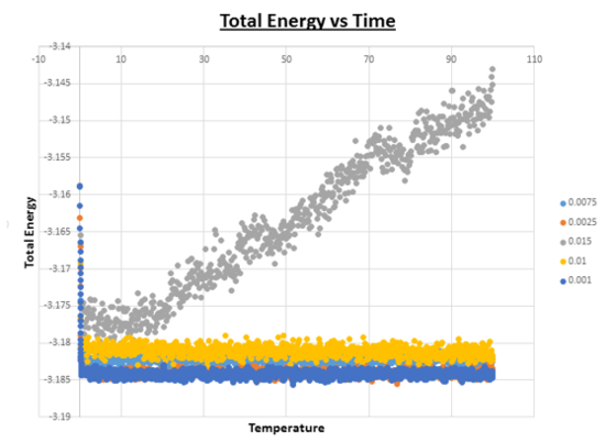
When you have done this, make a single plot which shows the energy versus time for all of the timesteps (again, attach a picture to your report).

|

Of the five timesteps that you used, which is the largest to give acceptable results? Which one of the five is a particularly bad choice? Why?

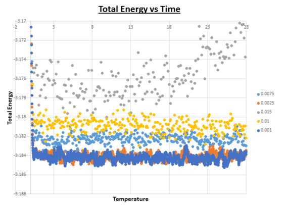
From looking at the combined ‘Total Energy vs Time’ graph, it is clear that the timestep which gives particularly bad results is the one with the largest timestep value (0.015). From first appearances (the graph above), it seems like all timesteps apart from 0.015 provide accurate data, because the energy reaches an equilibrium at an early stage of the simulation. However upon expansion of the energy axis, it is possible to see that there are differences.

|

Looking at this graph it can be seen that the average value of the energy ~ -3.184 for both the simulations with timesteps = 0.0025 and 0.001. As the value for the timestep is further increased, the average value of the energy increases. The greater the value of the timestep, the greater the value of the average energy. However as soon as the timestep is increased to 0.015 no equilibrium exists, and the average energy starts to fluctuate and increases as the simulation progresses. It is important for the energy average to stay constant throughout the simulation, if this is not the case, then the code on which the simulation is based needs to be adapted. Another feature of this graph that needs to be pointed out, is the degree of oscillation around the average. As the timestep is increased in value, we see a corresponding increase in oscillation about the average value as the timestep is increased. Ideally it is better to have as little oscillation as possible. In theory one would thus predict that the smaller the timestep, the better the results. However, the smaller the timestep, the shorter the overall simulation time we can compute. Therefore, an appropriate choice in the value of the timestep needs to be made, depending on the nature of the experiment.The largest timsestep to give acceptable results is 0.0025.

Running Simulations Under Specific Conditions

TASK: Choose 5 temperatures (above the critical temperature T^* = 1.5 ), and two pressures (you can get a good idea of what a reasonable pressure is in Lennard-Jones units by looking at the average pressure of your simulations from the last section). This gives ten phase points — five temperatures at each pressure. Create 10 copies of npt.in, and modify each to run a simulation at one of your chosen points. You should be able to use the results of the previous section to choose a timestep. Submit these ten jobs to the HPC portal. While you wait for them to finish, you should read the next section.

The 2 pressures that were chosen, were based on the results of the simulations of the previous section. Looking at the pressure vs time graph, it was evident that the equilibrium pressure was ~ 2.5. The values we therefore chose were determined with this in mind. We selected one of the pressures to be 2.5 and the other to have a similar value (2.7). All temperatures used were above the critical temperature (but not of a significantly higher value). The temperatures that were chosen were 1.6, 2.0, 3.0, 5.0 and 7.5. Five simulations were run with (each temperature once) and a temperature of 2.5 Another five simulations were run with the same temperatures but this time with the other pressure (2.7). The value of the timestep was chosen based based on the results of the previous section. Knowing that for a timestep value of 0.001, good results were obtained with no significant oscillation around the average, this was the value we used in all 10 simulations.

|

TASK: Use the manual page to find out the importance of the three numbers 100 1000 100000. How often will values of the temperature, etc., be sampled for the average? How many measurements contribute to the average? Looking to the following line, how much time will you simulate?

The three numbers are important in the sense that they tell you how the average is calculated of each property. In part 5 of this lab, we determined the heat capacity. One of the commands we used in the input file read as follows:

 fix aves all ave/time 100 1000 100000 v_dens v_temp v_press v_dens2 v_temp2 v_press2 v_etotal v_etotal2

 run 100000

This command instructs LAMMPS how to compute the average for the different properties we are interested in (density, temp, pressure, dens^2, temp^2, etotal, and etotal^2). The numbers 100 1000 100000 tells LAMMPS to take a sample 100 steps, the second number tells LAMMPS how many samples to take (in this case 1000). The final number (100000) tells us how long the simulation runs before an average is taken. So to sum up what the entirety means, ‘every 100 steps a sample is taken, until 100000 steps is reached, in total 1000 samples are taken, these 1000 samples are then averaged, and a single average value is determined.’ If the simulation time is also 100000 and thus equal to the last number of the fix aves command, 1 average will be generated. Increasing the total simulation time, can thus increase the amount of averages generated.

Looking to the following line, how much time will you simulate?

100000

Plotting the Equations of State

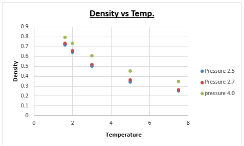
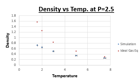
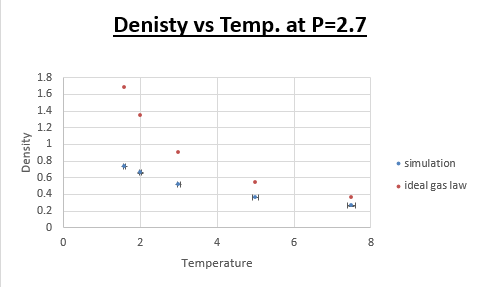
TASK: When your simulations have finished, download the log files as before. At the end of the log file, LAMMPS will output the values and errors for the pressure, temperature, and density \left({\frac {N}{V}}\right). Use software of your choice to plot the density as a function of temperature for both of the pressures that you simulated. Your graph(s) should include error bars in both the x and y directions. You should also include a line corresponding to the density predicted by the ideal gas law at that pressure. Is your simulated density lower or higher? Justify this. Does the discrepancy increase or decrease with pressure?

|

The formula above illustrates that a larger mean fee path is expected when the temperature is raised. This leads to less collisions per timestep, meaning that overall there is less potential energy between atoms. This results in ideal gas law being a better fit at higher temperatures (because ideal gas law assumes there is no potential energy between atoms) when making a direct comparison between the data points of the simulation and ideal gas law data.

|

Is your simulated density lower or higher? Justify this

Lower. The equilibrium distance for the ideal gas is lower than that for the simulation. Therefore the density will be higher at the same conditions. Due to the fact that in the ideal gas law we assume there to be no potential energy, as a result atoms can approach one another closer than is the case in a 'real' system. This stems from the fact that there is a significant repulsive component in the Lennard-Jones potential, at small internuclear separations.

Does the discrepancy increase or decrease with pressure?

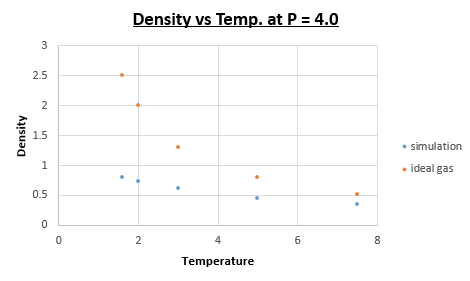
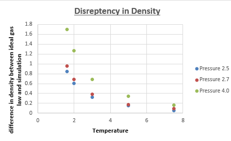
Graphically it was difficult to see whether the disrepancy increased or decreased as a function of pressure. Therefore a new series of simulations was run, this would not only make a possible trend more evident, but it would also make the proposed trend more reliable (3 pressures is more reliable than 2 pressures). We chose a pressure of 4, and kept all other variables (timestep, temperature, ensemble etc.) the same. The difference between the ideal gas density and the density calculated from the simulation were plotted for all 3 pressures.

|

This graph clearly illustrates that as the pressure is increased, the deviation between ideal gas law, and the density determined by the simulation becomes greater. Intuitively this makes sense, because the simulation is a better approximation of the 'actual' density than is the ideal gas law. Knowing that ideal gas law becomes more accurate at low pressures (the assumption that atoms don't interact is better at low pressures, where molecules are further apart), we can therefore predict that at lower pressures, we will get a better fit for the density as a function of temperature between ideal gas law and the density determined by the simulations.

Calculating Heat Capacities Using Statistical Physics

Heat Capacity Calculation

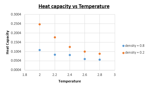
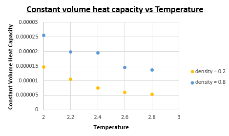
TASK: As in the last section, you need to run simulations at ten phase points. In this section, we will be in density-temperature (P*, T*) phase space, rather than pressure-temperature phase space. The two densities required at 0.2 and 0.8, and the temperature range is 2.0, 2.2, 2.4, 2.6, 2.8. Plot Cv as a function of temperature for both of your densities (on the same graph). Is the trend the one you would expect? Attach an example of one of your input scripts to your report.

Example input file: here

|

Upon dividing the heat capacity we obtain from the output data with the volume of the 'box' we can determine the constant volume heat capacity.

|

As we can see from the constant volume heat capacity vs Temperature plot the constant volume heat capacity increases as the density is increased. We also notice a decrease in constant volume heat capacity as the temperature is increased.

Is the trend the one you would expect?

Yes the trend is what we expect it to be. Increasing the density is accompanied with an increase in constant volume heat capacity, this is intuitive considering that we have a constant amount of atoms, we know that an increase in density must mean a corresponding decrease in volume (which is what we obtain when we analyse the output data volume = 4218.78 for when the density = 0.8 and volume = 16869.59 for when the density = 0.2). A smaller volume with the same amount of atoms means a larger heat capacity. Knowing that every atom contributes a finite contribution to the heat capacity, we know that the more atoms there are in a given volume, there must be a larger heat capacity accompanied with that volume.

To explain why the constant volume heat capacity decreases as the temperature is increased, we need to understand intuitively what happens when all energy levels are equally occupied in a system. As T is increased, all energy levels are occupied with the same probability. As a result the system will become saturated (eventually (at T = infinity)) and thus be unable to absorb any more energy, which is why as T->infinity the heat capacity will tend to 0. Since we are analysing a system which doesn't take into account temperatures of this nature we cannot prove that it will indeed go to 0, but the decrease in heat capacity as a function of temperature is definitely evident.

Structural properties and the radial distribution function

Vapour

Density = 0.04 Temperature = 1.2

Liquid

Density = 0.8 Temperature = 1.2

Solid

Density = 1.6 Temperature = 0.4

Again we observe the calculation time to be higher as we increase the density (this is because there are more collisions), as a result, the calculation time order was as followed:

Vapour < liquid < solid

|

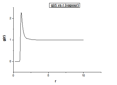
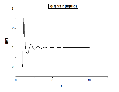
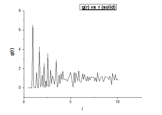
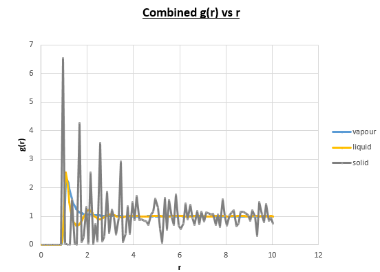
Below we illustrate the g(r) vs (r) plots obtained using the trajectory files obtained upon completing the simulations.⁴

|

The radial distribution function provides information of the radial characteristics of the atoms within a system. They are used to detect deviations with respect to the order of the crystal, which in this case has a cubic lattice type FCC.

g(r) provides detailed information on the radial characteristics of the atomic or particulate system under study while rotationally invariant measures detect orientational deviations with respect to perfect local order.

Discuss qualitatively the differences between the three RDFs, and what this tells you about the structure of the system in each phase.

We must first distinguish between solids, liquids, and gases. Solids: In particular crystals, display a regular and ordered structure. Liquids: motion of atoms is based on Brownian motion. Gases: Long free mean paths.

Assuming we are analysing a single atom within a system. In a solid, neighbouring atoms are found at characteristic distances. This can be described as ‘regular spacing.’ In a liquid state, atom spacing is irregular. Neighbouring atoms are not found at exact distances, instead they are found at approximate distances. Gases have a more irregular spacing. A more formal approach to determining how ordered a system is by making use of the radial distribution function. The radial distribution function describes the relative density of the atoms as a function of the radius. A more intuitive description would be to view the radial distribution function as the ratio between the local atom density and the overall atom density.

The differences between the different g( r ) vs r plots is the loss in the number of favoured distances. This can be explained by the fact order decreases from solid to vapour. In the vapour g( r ) vs r graph we still observe a single peak, how can this be explained? Even in the vapour phase there is a distance which is favoured by atoms, this is the equilibrium distance. Comparing the liquid g( r ) vs r graph to the corresponding vapour plot, we notice a few extra oscillations. This is because while atoms move around in a liquid, it is still a more ordered system than a vapour is.

What is the meaning of the peaks in a radial distribution vs radius graph?

The peaks illustrate a favoured separation between atoms. Intuitively, we would then expect well defined peaks for solids. Atoms within a solid don’t move much, and so we would expect the distances to be very specific, and thus expect narrow peaks. When looking at the g( r ) vs r graph for the fcc solid, we notice well defined peaks. However we also observe peaks which are not infinitely thin. To understand why this is so, we need to realise that while a solid crystal has a higher order, which consist of reproducible unit cells, a crystal is rarely perfect. As a result, the distances of a single atom to all its neighbouring atoms in the first neighbouring shell are not exactly the same. We therefore see peaks which are in actual fact a distribution over a small range of distances (a perfect crystal would just be a delta function. Between the different neighbouring shells, we expect distances at which the probability is equal to 0, assuming the crystal is perfect. However this is not the case unless the crystal is 100% perfect. As we move to greater distances we observe peaks with less significant intensities. This makes sense considering that the order decreases as a function of distance. The intensity of the peaks is also dependent on the nature of the lattice type. Different lattices will have different probabilities of finding a neighbouring atom at a given distance. By assuming that the solid can be described as a perfect FCC lattice, we can intuitively predict how many neighbouring atoms are in each neighbouring shell. It turns out that for an FCC lattice type, the neighbouring spheres consist of 12, 6, 24, and 12 atoms respectively in the first 4 neighbouring shells.³

Why are there inevitably defects in crystals?

This stems from the fact that defects cause an increase disorder, which leads to an increase in the number of microstates available to the system. As a result, entropy will increase which is a favourable process. Apart from the fact that it is inherently difficult to obtain a crystal that is 100 % pure (due to possible contaminants coming from a large number of sources), there is thus also a thermodynamic driving force which causes crystals to be imperfect.

Why does a g( r ) vs r graph level off when we go to large values for r?

Going to larger distances, order decreases. Assuming we are observing a single atom within a crystal, and observing only the 4th nearest neighbours. Intuitively we can predict that the distance for all these 4th nearest neighbours should be equal in a perfect crystal. However due to the inevitable presence of defects, we can predict that the probability of finding a defect, and thus finding a defect along its path, is higher, the longer the distance is between your atoms. On the assumption that every defect will cause a discrepancy in the value for the distance between the observed atom and the 4th nearest neighbours we can predict a larger error for the 4th nearest neighbours, compared to neighbours in closer proximity to the observed atom. Knowing that the distance gets bigger between the observed atom and the nth neighbour (as n increases), and that the peak width of a g( r ) vs r graph is a function of error, we can accurately conclude that for the FCC lattice we are analysing, the peak height decreases and the peak width increases as n is increased. Peak height decreasing, and peak width increasing directly leads to a flatting of the g( r ) vs r graph, as r is increased.

Pair correlation Function

This type of function only considers pairs of atoms. It is a very accurate measure in providing structural information. It does a particularly good job in describing the structure and nature of liquid systems.

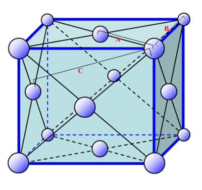
In the solid case, illustrate which lattice sites the first three peaks correspond to.

|

As is labelled in the figure above, the 3 smallest distances (from which all distances are referenced) are denoted A, B and C. In this case A is the smallest distance and refers to the first closest neighbours (first peak), B is the second smallest distance and refers to the second closest neighbours (second peak) and C is the third smallest distance and refers to the third closest neighbours (third peak).

What is the lattice spacing?

The first maximum tells you with a good approximation where the nearest neighbour is. Since we know we are dealing with an FCC lattice, we know that the second nearest neighbour is located at exactly one lattice parameter away. By observing the location of the second maximum peak on the g(r) vs r (solid) graph, we find that this peak is found at r = 1.35, which as a result is also equal to our lattice spacing.

What is the coordination number for each of the first three peaks?

|

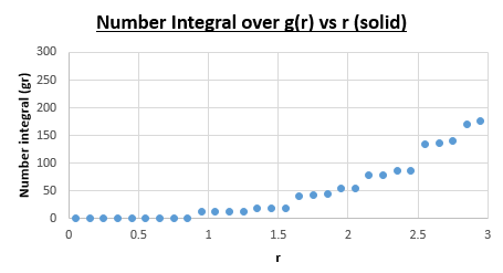
For the first nearest neighbour we can find the coordination number by looking at the value of r where the first peak collapses, which is at r = 1.05. The running integral at this value for r is equal to exactly 12. For the second nearest neighbours the second peak collapses at 1.45. The running integral at this value for r gives 18. Due to the fact that we are dealing with a running integral, we must substract the area of first peak, which gives 18-12 = 6. The coordination number of the second nearest neighbour is therefore 6. The third peak (corresponding to the third nearest neighbours) on the g(r) vs (r) solid plot collapses at r = 1.75. Looking at the number integral over g(r) vs r (solid) plot at r = 1.75 gives a value of 42 for the integral. Subtracting 18 from 42 gives 24. The coordination number of the third nearest neighbours is thus 24.

In conclusion this gives coordination numbers of 12, 6, and 24 for the first, second and third nearest neighbours respectively.

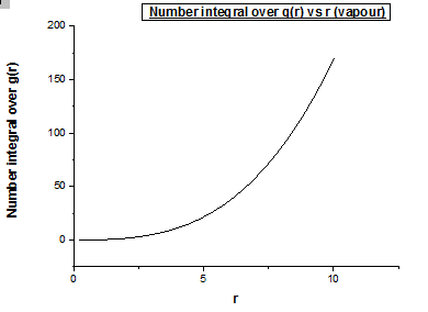
Bellow we also illustrate the number integral over g(r) vs r graphs for a vapour, liquid and solid of the Lennard Jones potential respectively.

|

Dynamical Properties and The Diffusion Coefficient

In this section we will make use of new concepts such as the mean squared displacement and the velocity autocorrelation function, which we can use to determine the diffusion coefficient.These diffusion coefficients were then compared to determine the validity of each approach.

| | | |

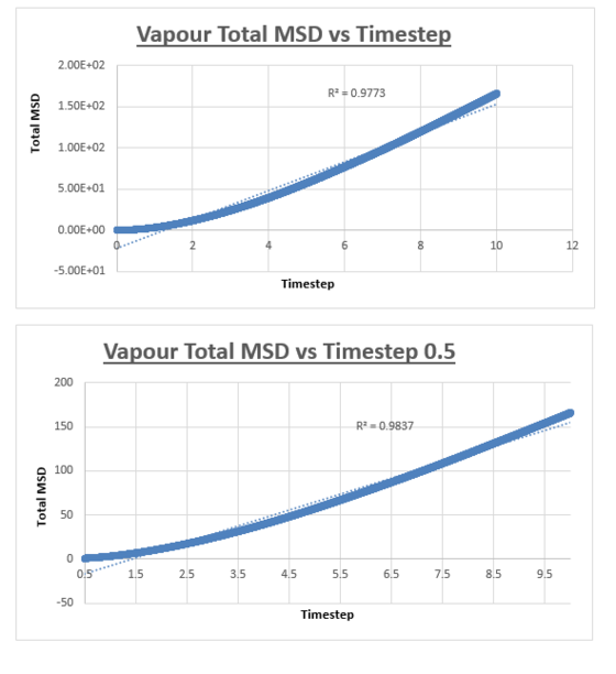
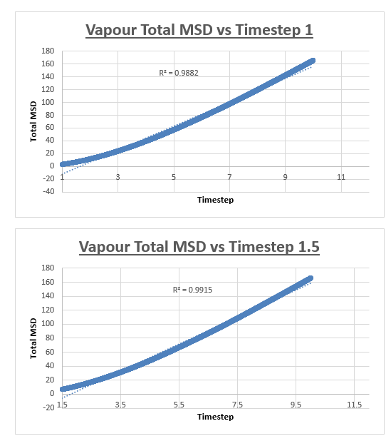
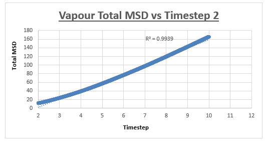
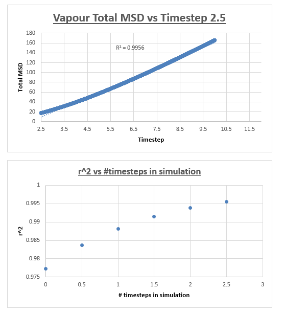
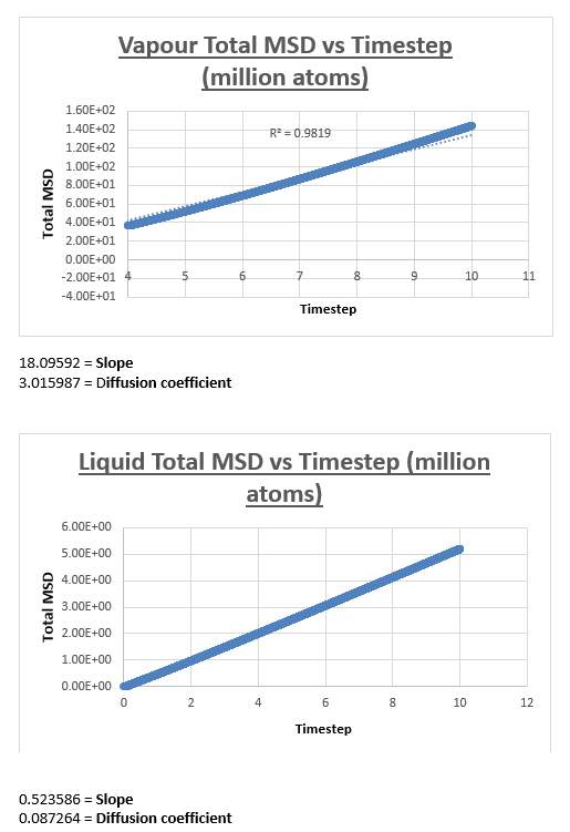
For the vapour MSD vs time step graph, the graph did not appear linear from start to finish. We therefore evaluated the slope of the graph from various starting points, analysing the r2 value of each of the trendlines respectively. These r2 values were then plotted as a function of the different starting points. The r2 value appeared to converge, we therefore decided to measure the slope of the MSD vs time step graph, from the timstep where the r2 started to converge. In the case of the vapour, we decided that taking the trendline from the timestep = 2.5 to the end of the simulation would give an accurate enough result. The shape of the graph was what we expected, in the vapour phase we expect a linear relation between the MSD and the timestep. However upon close inspection we notice that at small values for the timestep, the relation is not linear. This can be explained by the fact that an atoms movement will follow a straight line until it collides with another atom. Once the atom has collided with another atom, can its path be described by a random walk. In the very beginning of the simulation, the atom will not have collided with another atom, we can therefore assume it is moving at a constant velocity. This effectively means that the distance travelled is proportional to time. Since the MSD is the mean squared distance, we expect it to be proportional to the square of the time. This is why we observe a parabolic shape of the graph at the very beginning of the simulation.

The slope of this trendline was determined to have a value of 20.156

The diffusion coefficient is therefore 3.359

Liquid

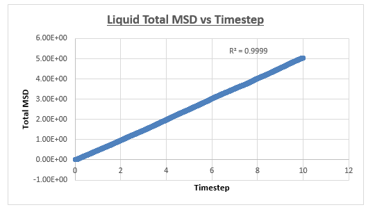
The MSD vs timestep graph for the liquid appeared to be linear, which was confirmed by the r2 value. We therefore drew a trendline across the whole simulation. The diffusion coefficient was then consequently found by multiplying this number by 1/6. The shape of the graph is what we expect it to be (linear), in a liquid atoms are in closer proximity and thus relatively to gas atoms in constant contact with each other. Therefore it’s not strange for us to observe a continuous linear relationship in the total MSD vs timestep graph.

|

The slope of this trendline was determined to have a value of 0.509

The diffusion coefficient is therefore 0.0849

Solid

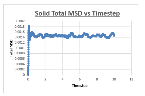
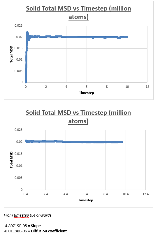
The MSD vs timestep graph for a solid appeared to be completely different from the MSD vs timestep graph obtained for both the liquid and vapour. Initially we see a sudden rise in total MSD, which then levels off with no further increase observed as the simulation is progressed. To explain the nature of the graph, we must first understand the meaning of the total MSD. Often defined as the ‘spatial extent of motion,’ we can understand the total MSD of a solid by imagining a solid where all atoms are ordered, and where movement is limited. An atom within this solid has only a finite amount of space it can move in. Once the atom has ‘explored’ all the area it can move in, the total MSD levels off and does not increase any further, which is what we observe in the graph below.

|

The slope of this graph is taken from 0.5 (timestep) to the end of the simulation, taken the slope from the slope by drawing a trendline from beginning to end would results in an inaccurate value for the diffusion coefficient.

The value for the slope was found to be 7.6204E-09.

As a result, the value for the diffusion coefficient was found to be 1.27007E-09

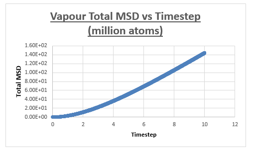
One million atom simulations

Vapour

| | |

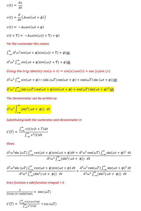
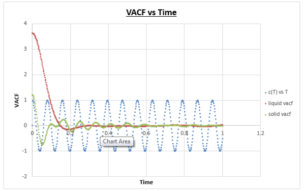
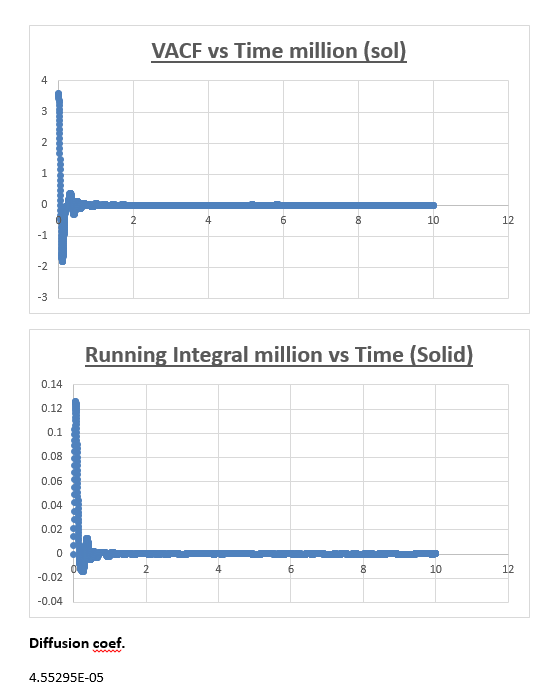
Task: Be sure to show your working in your write-up. On the same graph, with x range 0 to 500, plot with and the VACFs from your liquid and solid simulations. What do the minima in the VACFs for the liquid and solid system represent? Discuss the origin of the differences between the liquid and solid VACFs. The harmonic oscillator VACF is very different to the Lennard Jones solid and liquid. Why is this? Attach a copy of your plot to your writeup.

|

Task: What do the minima in the VACFs for the liquid and solid system represent?

The minimum is reached when the velocity vectors are anti-parallel to one another, within the time t+T the vector needs to have become anti-parallel. When this occurs the difference in velocity of t and t+T is the lowest. Intuitively in our system we can imagine this occurring when the atoms collide against one another. For a liquid, beyond a minimum the shape of the graph can be described by atoms that have just collided (minimum) causing the atoms to bounce away from one another and consequently allowing them to diffuse away from one another.

Task: Discuss the origin of the differences between the liquid and solid VACFs.

Solids and liquids are systems where the interatomic forces are inherently strong. Atoms in such systems tend to take up positions where there is a balance between repulsive and attractive forces, because this minimises the energy. Due to the fact that in a solid these positions are even more stabilising than in a liquid, the movement of atoms can be described by vibrations. These vibrations can be described as an oscillation where the atoms move one way and move back in the opposite direction, leading to a reversal of the velocity vector. It is for this reason that when we observe the solid VACF vs timestep graph that we observe continuous oscillation. Similarly to a gas and a liquid, the VACF goes to zero as long as we extend the time to a high enough value. It should be noted that while we observe a set of oscillations in the VACF vs time graph of the solid, these oscillations decrease in magnitude as the simulation time increases. This can be explained by taking account forces which causes a disturbance to the atoms (a so-called perturbation). Liquids and solids are different in the sense that in a liquid atoms do not have fixed positions. As a result diffusion plays a much bigger role. In a sense diffusion rids the VACF from oscillating over time. As a result we don’t observe continuous oscillation over time, but instead we observe an oscillation which is damped (a single minima).⁵

Task: The harmonic oscillator VACF is very different to the Lennard Jones solid and liquid. Why is this?

For the VACF one side of the function is favoured over the other because the potential is non symmetrical. The function is directional when this model is used and therefore there is a change happening of the velocity, if there is change happening, c(t) will also decrease unlike for the simple harmonic oscillator which is fully symmetrical. This is why we observe a damping effect for the Lennard-Jones plots and not for the harmonic oscillator VACF.

Trapezium Rule

|

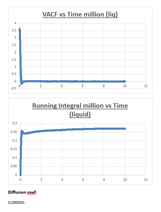
Million Atoms

|

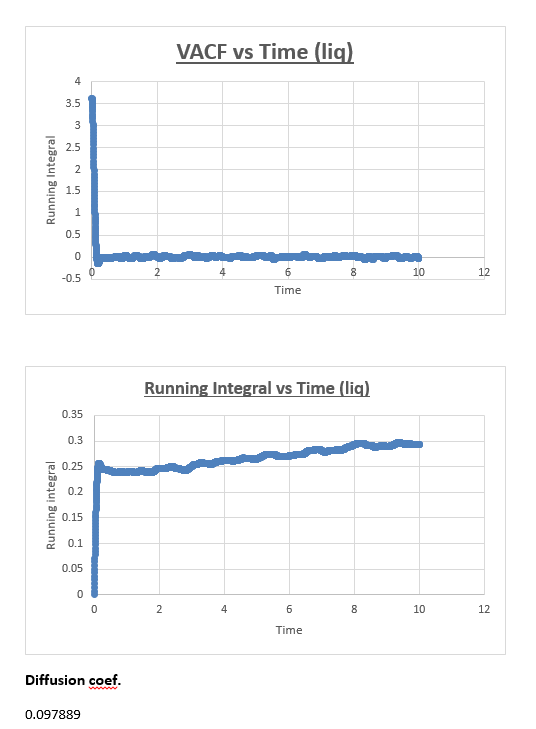
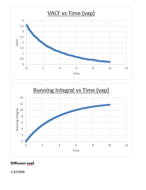
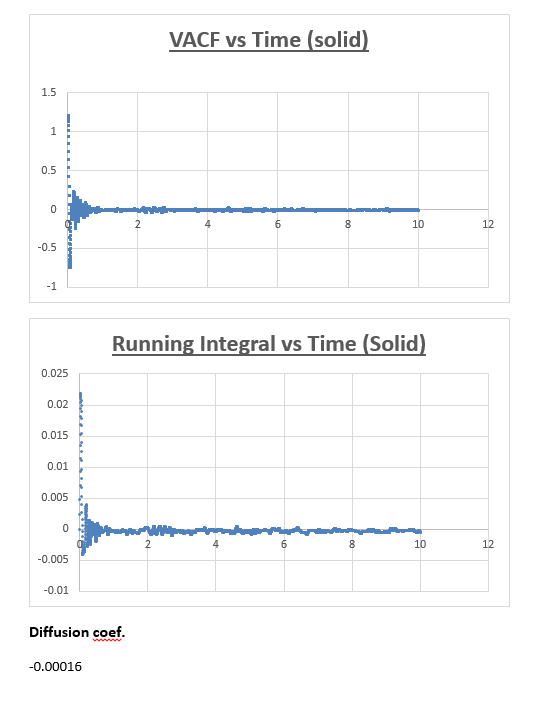
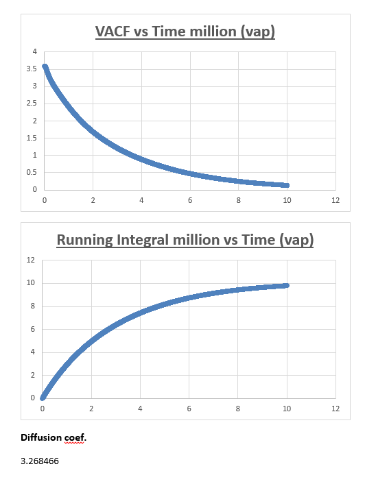
You should make a plot of the running integral in each case. Are they as you expect?

The running integral plot is what we expect it to be. This is proven by taken a look at the last value obtained for the running integral, dividing this number by 3 gives a diffusion coefficient for the vapour, liquid and solid which is very similar to the diffusion coefficient we obtained from the MSD vs timestep plots.

What do you think is the largest source of error in your estimates of D from the VACF?

Estimating the diffusion coefficient using trapezium rule is the biggest source of error. Trapezium rule is only an approximation to the true integral.We assumed the width of our rectangles to be half of 0.002 (0.001). The greater the slope within this timeframe the greater the error will be. One way of reducing the error would be to make the rectangles infinitesimally thin in width. Eitherway our calculation of the diffusion coefficient from the VACF is reasonably accurate considering it is similar in nature to the respective diffusion coefficient we obtained from the mean squared displacement.

Bibliography

1) (http://ecee.colorado.edu/~bart/book/fcc.gif (accessed 7/02/14))

2) (http://ecee.colorado.edu/~bart/book/bravais.htm 7/02/14))

3) (http://ocw.mit.edu/courses/materials-science-and-engineering/3-021j-introduction-to-modeling-and-simulation-spring-2012/part-i-lectures-readings/MIT3_021JS12_P1_L4.pdf 7/02/14))

4) J. Hansen and L. Verlet, Physical Review, 1969, 184, 151.

5) (The Velocity Autocorrelation Function http://www.ccp5.ac.uk/DL_POLY/Democritus/Theory/vaf.html 8/02/14)