Rep:Mod:lb3714liquidsim

Introduction to Molecular Dynamics Simulation

Figure 1: Particle position over time for a timestep of 0.1.

Figure 2: Total energy over time for a timestep of 0.1.

Figure 3: Absolute error between manually calculated position and that calculated using the velocity Verlet algorithm.

Experimenting with timestep values

Timestep	ΔE (%)
0.001	0.000
0.010	0.001
0.050	0.031
0.100	0.125
0.150	0.281
0.200	0.500
0.250	0.781
0.300	1.125
0.500	3.125
1.000	9.375

Figure 4: Error maxima as a function of time for a timestep of 0.1.

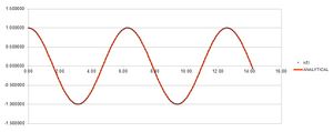
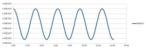
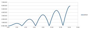
The table above shows that a timestep of approximately 0.25 or less is needed to ensure the total energy does not change by more than 1% over the course of the simulation. It is important to monitor total energy throughout a simulation because energy is conserved; that is, total energy is constant. If it changes significantly during the course of a simulation, the simulation will not accurately reflect reality.

Atomic Forces

Lennard-Jones potential

$V=4ϵ(\frac{{\sigma }^{12}}{r^{12}}-\frac{{\sigma }^6}{r^6})$

When the potential energy is zero, $r_0=\sigma$.

At equilibrium, the force, $F_i$ is zero, so the minimum must be found.

$F_i=-\frac{dV}{dr}=-4ϵ(\frac{-12{\sigma }^{12}}{r^{13}}-\frac{6{\sigma }^6}{r^7})=0$

$\frac{48ϵ{\sigma }^{12}}{r^{13}}=\frac{24ϵ{\sigma }^6}{r^7}$

$\frac{48ϵ{\sigma }^{12}}{24ϵ{\sigma }^6}=\frac{r^{13}}{r^7}$

$2{\sigma }^6=r^6$

$r_{eq}={\sigma }^6\sqrt{2}=1.122\sigma$

Well depth at $\varphi (r_{eq})$:

$4ϵ(\frac{{\sigma }^{12}}{{(}^6\sqrt{2}\sigma {)}^{12}})-(\frac{{\sigma }^6}{{(}^6\sqrt{2}\sigma {)}^6})$

$4ϵ(\frac{{\sigma }^{12}}{4{\sigma }^{12}})-(\frac{{\sigma }^6}{2{\sigma }^6})$

$4ϵ(\frac{1}{4})-(\frac{1}{2})$

$4ϵ(-\frac{1}{4})$

$-ϵ$

Evaluating integrals when $ϵ=\sigma =1$:

$\varphi (r)=4(\frac{1}{r^{12}}-\frac{1}{r^{12}})$

$\int \varphi (r)=-\frac{4}{11r^{11}}+\frac{4}{5r^5}$

$\underset{2}{\overset{\mathrm{\infty }}{\int }}\varphi (r)=(-\frac{4}{11{\mathrm{\infty }}^{11}}+\frac{4}{5{\mathrm{\infty }}^5})-(-\frac{4}{11(2{)}^{11}}+\frac{4}{5(2{)}^5})$

$(-\frac{4}{11{\mathrm{\infty }}^{11}}+\frac{4}{5{\mathrm{\infty }}^5})⟶0$, therefore:

$\underset{2}{\overset{\mathrm{\infty }}{\int }}\varphi (r)=\frac{4}{11(2{)}^{11}}-\frac{4}{5(2{)}^5}=-2.482\times 10^{-2}$

$\underset{2.5}{\overset{\mathrm{\infty }}{\int }}\varphi (r)=\frac{4}{11(2.5{)}^{11}}-\frac{4}{5(2.5{)}^5}=-8.176\times 10^{-3}$

$\underset{3}{\overset{\mathrm{\infty }}{\int }}\varphi (r)=\frac{4}{11(3{)}^{11}}-\frac{4}{5(3{)}^5}=-3.290\times 10^{-3}$

Periodic Boundary Conditions

Number of water molecules in 1 mL of water under standard conditions:

$V=1c{m}^3$

$\rho =1gc{m}^{-3}$

$Mass=1g$

$Moles=\frac{1}{18}=0.05$

$Numberofmolecules=0.05\times 6.022\times 10^{23}=3.346\times 10^{22}$

Volume of 10,000 water molecules:

$\frac{10,000}{6.022\times 10^{23}}=1.66\times 10^{-20}moles$

$Volume=1.66\times 10^{-20}\times 18=2.99\times 10^{-19}c{m}^3$

If an atom at position $(0.5,0.5,0.5)$ moves along the vector $(0.7,0.6,0.2)$, after the periodic boundary conditions have been applied it would end up at the position $(0.2,0.1,0.3)$.

Reduced Units

$r^{*}=3.2$, $\frac{ϵ}{k_B}=120K$

$r=3.2\times 0.34=1.088nm$

$ϵ=120K\times 8.314J{K}^{-1}mo{l}^{-1}=998Jmo{l}^{-1}=0.998kJmo{l}^{-1}$

$T=120\times 1.5=180K$

Equilibriation

Creating the Simulation Box

Giving atoms random starting coordinates and subsequently generating two atoms close together could cause the atoms to merge into each other.

In a simple cubic lattice, there is 1 atom. If the lattice spacing is 1.07722:

$\frac{1}{1.07722^3}=0.79999=0.8$

In a face-centred cubic lattice, there are 4 atoms. If the density is 1.2, the lattice spacing is approximately 1.4938:

$\frac{4}{a^3}=1.2$

$a^3=\frac{4}{1.2}=\frac{10}{3}$

$a{=}^3\sqrt{\frac{10}{3}}=1.4938$

If a face-centred cubic lattice had been defined instead, 4000 atoms would have been created, since such a lattice contains 4 atoms.

Setting the properties of the atoms

Script	Definition
mass 1 1.0	Sets the mass for all atoms of one or more atom types. The first number corresponds to atom type, which is arbitary; the second number corresponds to the mass of the type.
pair_style lj/cut 3.0	Sets the formulae LAMMPS uses to compute pairwise interactions. Here, lj corresponds to the style, and cut 3.0 corresponds to the arguments used by that style.
pair_coeff * * 1.0 1.0	Specifies the pairwise force field coefficients for one or more pairs of atom types. The asterisks represent atom types, and 1.0 1.0 (arguments) represent the coefficients for the pairs, which depend on the pair style.

Since we are specifying $x_i(0)$ and $v_i(0)$, we are using the Velocity Verlet Algorithm.

Running the Simulation

### SPECIFY TIMESTEP ###
variable timestep equal 0.001
variable n_steps equal floor(100/${timestep})
variable n_steps equal floor(100/0.001)
timestep ${timestep}
timestep 0.001

### RUN SIMULATION ###
run ${n_steps}
run 100000

The purpose of n_steps is to simulate how much time to run (100) and to divide it into timesteps. Simply writing

timestep 0.001
run 100000

indicates the number of timesteps to run, but not actually the amount of time.

Checking Equilibriation

Figure 5: Total energy vs time for a timestep of 0.001.

Figure 6: Temperature vs time for a timestep of 0.001.

Figure 7: Pressure vs time for a timestep of 0.001.

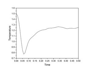
The simulation reaches pressure equilibrium after approximately 0.2 seconds, and energy and temperature equilibrium after approximately 0.3 seconds.

Figure 8: Plots of total energy vs time for different timesteps.

The largest timestep to use that gives acceptable results is 0.0025. At timesteps above this, the values for energy, temperature and pressure begin to diverge (which may yield inaccurate values), whereas values for 0.001 and 0.0025 are very similar. Conversely, 0.015 is a particularly bad timestep to use because it does not equilibriate within the time specified.

Running Simulations Under Specific Conditions

Examining the Input Script

fix aves all ave/time 100 1000 100000 v_dens v_temp v_press v_dens2 v_temp2 v_press2

fix ave/time, the command on this line of script, takes one or more input values every few timesteps and averages them over longer timescales. The general fix ave/time command takes the following form:

fix ID group-ID ave/time Nevery Nrepeat Nfreq value1 value2 ... keyword args ...

In this simulation:

• Nevery = 100, meaning that input values are sampled every 100 timesteps.
• Nrepeat = 1000, meaning that input values are used to calculate averages 1000 times over the course of the simulation.
• Nfreq = 100000, meaning that averages are calculated every 100000 timesteps.

100000 timesteps will be simulated.

Chosen Conditions

Conditions were chosen by looking at the average values gained in the previous simulations. A timestep of 0.0025 was used.

Temperatures:

• 2.50
• 3.00
• 3.50
• 4.00
• 5.00

Pressures:

Figure 9: Pressure values for the first five simulations.

The following pressures were selected because the previous simulations showed an average pressure of about 2.5.

• 2.00
• 3.00

Thermostats and Barostats

$\frac{1}{2}\sum m_i{v}_i^2=\frac{3}{2}N{k}_{B}T$

$\frac{1}{2}\sum m_i(\gamma v_i{)}^2=\frac{3}{2}N{k}_B\mathfrak{𝔗}$

The value of $\gamma$ calculated so that the temperature is correct $T=\mathfrak{𝔗}$ if we multiply every velocity by $\gamma$ was calculated as follows:

$\frac{1}{2}\sum m_i{\gamma }^2{v}_i^2=\frac{3}{2}N{k}_B\mathfrak{𝔗}$

$\frac{1}{2}{\gamma }^2\sum m_i{v}_i^2=\frac{3}{2}N{k}_B\mathfrak{𝔗}$

Since $\frac{1}{2}\sum m_i{v}_i^2=\frac{3}{2}N{k}_{B}T$:

$\frac{3}{2}{\gamma }^{2}N{k}_{B}T=\frac{3}{2}N{k}_B\mathfrak{𝔗}$

${\gamma }^{2}T=\mathfrak{𝔗}$

${\gamma }^2=\frac{\mathfrak{𝔗}}{T}$

$\gamma =\sqrt{\frac{\mathfrak{𝔗}}{T}}$

Results and Discussion

Figure 10: Relationship between temperature and simulated density for both pressures.

Figure 11: Comparison between simulated density and that calculated using the ideal gas law for a pressure of 2.

Figure 12: Comparison between simulated density and that calculated using the ideal gas law for a pressure of 3.

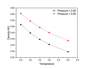
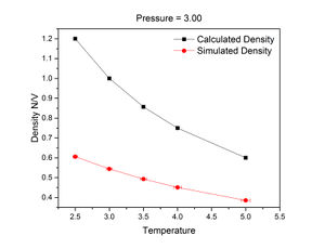
The figures on the right show that for both pressures, density decreases with temperature. At all temperatures, density was higher at a pressure of 3 than 2. Predicted density was calculated from the following variant of the ideal gas law:

$\frac{P}{k_{b}T}=\frac{N}{V}$

Where $k_b$, the Boltzmann constant, was assumed to = 1 as is standard in LAMMPS.

The density trends calculated using the ideal gas law were significantly higher than the relevant simulated trends. This is because the ideal gas law calculates density using bulk volume, which does not take voids into account and so assumes a 100% packing efficiency. In the simulation, the initial structure of the crystal was a simple cubic lattice, which has a packing efficiency of about 52%. This is further evidenced by the ratio between the simulated and calculated densities at a pressure of 3 and temperature of 2.5:

$\frac{Simulated}{Calculated}=\frac{0.69}{1.29}=0.5349=53\mathrm{\%}$

However, the discrepancy between simulated and calculated densities decreased with pressure.

Calculating Heat Capacities using Statistical Physics

Figure 13: Relationship between temperature and heat capacity for two densities.

Example script

### DEFINE SIMULATION BOX GEOMETRY ###
variable dens equal 0.2
lattice sc ${dens}
region box block 0 15 0 15 0 15
create_box 1 box
create_atoms 1 box

### DEFINE PHYSICAL PROPERTIES OF ATOMS ###
mass 1 1.0
pair_style lj/cut/opt 3.0
pair_coeff 1 1 1.0 1.0
neighbor 2.0 bin

### SPECIFY THE REQUIRED THERMODYNAMIC STATE ###
variable T equal 2.0
variable p equal 1.0
variable timestep equal 0.0025

### ASSIGN ATOMIC VELOCITIES ###
velocity all create ${T} 12345 dist gaussian rot yes mom yes

### SPECIFY ENSEMBLE ###
timestep ${timestep}
fix nve all nve

### THERMODYNAMIC OUTPUT CONTROL ###
thermo_style custom time etotal temp press
thermo 10

### RECORD TRAJECTORY ###
dump traj all custom 1000 output-1 id x y z

### SPECIFY TIMESTEP ###

### RUN SIMULATION TO MELT CRYSTAL ###
run 10000
unfix nve
reset_timestep 0

### BRING SYSTEM TO REQUIRED STATE ###
variable tdamp equal ${timestep}*100
variable pdamp equal ${timestep}*1000
fix nvt  all nvt  temp ${T} ${T} ${tdamp}
run 10000
reset_timestep 0
unfix nvt
fix nve all nve

### MEASURE SYSTEM STATE ###
thermo_style custom step etotal temp press density atoms vol
variable n equal atoms
variable etotal equal etotal
variable etotal2 equal etotal*etotal
variable dens equal density
variable dens2 equal density*density
variable temp equal temp
variable temp2 equal temp*temp
variable press equal press
variable press2 equal press*press
variable vol equal vol
fix aves all ave/time 100 1000 100000 v_dens v_temp v_press v_dens2 v_temp2 v_press2 v_etotal v_etotal2
run 100000

variable avedens equal f_aves[1]
variable avetemp equal f_aves[2]
variable avepress equal f_aves[3]
variable errdens equal sqrt(f_aves[4]-f_aves[1]*f_aves[1])
variable errtemp equal sqrt(f_aves[5]-f_aves[2]*f_aves[2])
variable errpress equal sqrt(f_aves[6]-f_aves[3]*f_aves[3])
variable heatcap equal ${n}*${n}*(f_aves[8]-f_aves[7])/f_aves[5]

print "Averages"
print "--------"
print "Volume: ${vol}"
print "Heat capacity: ${heatcap}"
print "Density: ${avedens}"
print "Stderr: ${errdens}"
print "Temperature: ${avetemp}"
print "Stderr: ${errtemp}"

Results and discussion

The heat capacity for a density of 0.8 was greater than that for 0.2 at all temperatures. The heat capacity at a density of 0.8 plateaued at temperature ranges of 2.2-2.4 and 2.4-2.6; this could correspond to phase transitions. The trend established is not the one expected; theoretically the heat capacity should be expected to increase with temperature, but the established trend shows a decrease in $\frac{C_V}{V}$ with temperature. Also,higher densities should correspond to lower specific heat capacities; this is because at a higher density, the amount of heat a structure can intake is smaller.

The input script indicates that once the correct thermodynamic conditions have been established, the canonical ensemble NVT should be unfixed and the microcanonical ensemble NVE should be fixed. NVE assumes that energy E is constant; however, the calculation for heat capacity requires that the energy vary. Therefore, the discrepency between the theoretical trend between heat capacity and temperature, and the simulated trend, may be because during the simulation the total energy was taken to be constant, and so heat capacity and temperature were directly inverse to one another. In theory, the total energy should increase with temperature.

Structural Properties and the Radial Distribution Function

The radial distribution function g(r) describes how density varies as a function of distance from a reference particle. It describes how, on average the atoms in a system are radially packed around each other, allowing the average structure to be determined. RDF is usually plotted as a function of r, the interatomic separation.

Chosen conditions for simulation

	Solid	Liquid	Vapour
Density	1.20	0.80	0.05
Temperature	1.20	1.20	1.20

Results and discussion

Figure 14: Radial distribution functions for each phase.

The peaks in a radial distribution function represent probabilities that atoms lie at the location specified by r. The g(r) for the gas phase shows a peak when 1<r<2, but there is no significant oscillation at longer distances. The liquid g(r) shows some weak oscillation up to an rof 4. The solid g(r) shows strong oscillation peaks even at longer distances. This indicates the presence of long-range order consistent with a crystalline structure. In contrast, the gas g(r) shows only short-range order consistent with a highly disordered structure.

The crystal structure of the solid is a face-centred cubic lattice. The first peak in the radial distribution function corresponds to

Dynamical Properties and the Diffusion Coefficient

Mean Squared Displacement

Figure 15: Mean squared displacement vs timestep for each phase composed of 8000 atoms.

Figure 16: Mean squared displacement vs timestep for each phase composed of 1 million atoms.

Figure 17: Mean squared displacement for the solid phase.

Figure 18: Fitted mean squared displacement for the liquid phase.

Figure 19: Fitted mean squared displacement for the vapour phase.

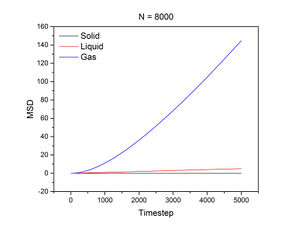
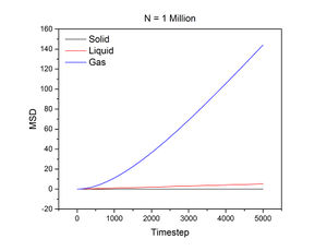
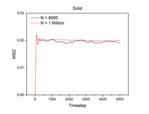
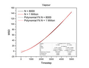
The conditions specified for each phase were the same ones for the previous section. D, the diffusion coefficient, was calculated from the gradient of each plot using the following equation:

$D=\frac{1}{6}\frac{\partial ⟨r^2\left(t\right)⟩}{\partial t}$

N = 800:

	Solid	Liquid	Vapour
Slope	$0.00\times 10^0$	$1.02\times 10^{-3}$	$1.43\times 10^{-3}$
D	$0.00\times 10^0$	$1.70\times 10^{-4}$	$2.38\times 10^{-3}$

N = 1 million:

	Solid	Liquid	Vapour
Slope	$0.00\times 10^0$	$1.05\times 10^{-3}$	$1.50\times 10^{-3}$
D	$0.00\times 10^0$	$1.75\times 10^{-4}$	$2.50\times 10^{-3}$

The mean squared displacement measures how far a particle deviates from a reference position over time. Figures 15 and 16, as well as the above tables, show that the gradient of the mean squared displacement over time increases in the ascending order of solid, liquid and vapour. This is expected because the solid is highly dense and so its atoms cannot diffuse far from the reference point; indeed, the gradient for the solid mean squared displacement is approximately zero. In contrast, the plot for the vapour (Figure 19) phase has a much higher gradient once a linear relationship is established after approximately 20000 timesteps. The vapour phase is not particularly dense and so its atoms are able to diffuse much further from the reference point much more rapidly.

Velocity Autocorrelation Function

Evaluating the integral:

$C\left(\tau \right)=\frac{\underset{-\mathrm{\infty }}{\overset{\mathrm{\infty }}{\int }}v\left(t\right)v(t+\tau )\mathrm{d}t}{\underset{-\mathrm{\infty }}{\overset{\mathrm{\infty }}{\int }}{v}^2\left(t\right)\mathrm{d}t}$

$v(t)=\frac{dx(t)}{dt}$

$\underset{-\mathrm{\infty }}{\overset{\mathrm{\infty }}{\int }}v(t)=x(t)=ACos(\omega t+\varphi )$

Earlier the values for $A$ and $\varphi$ were given:

• $A$=1.00
• $\varphi$=0.00

Therefore $x(t)=Cos(\omega t)$.

$C(\tau )=\frac{Cos(\omega t)Cos(\omega t+\tau )}{Co{s}^2(\omega t)}$

$C(\tau )=\frac{Cos(\omega t+\tau )}{Cos(\omega t)}$

Figure 19: Velocity autocorrelation functions for the solid and liquid phases.

The velocity autocorrelation function indicates the difference in velocities of an atom will be between time $t$ and $t+\tau$; essentially how the velocity of the atom changes over time. A plot of the velocity autocorrelation function shows oscillation peaks corresponding to vibrations that weaken over time, indicating that interatomic forces are decaying the velocity. The minima represent a temporary lack of change in velocity as the atom slows down and speeds back up again. The plot for the solid shows more oscillation peaks than that for the liquid. This is because the intermolecular forces in a solid are much stronger and therefore have a larger effect on the velocity. The are therefore in good agreement with theory.

References

- ↑ Atkins, P. and De Paula, J., 2014. Atkins’ Physical Chemistry. New York, pp.12.
- ↑ Ginnings, D.C. and Furukawa, G.T., 1953. Heat Capacity Standards for the Range 14 to 1200° K. Journal of the American Chemical Society, 75(3), pp.522-52
- ↑ Alder, B.J. and Wainwright, T.E., 1970. Decay of the velocity autocorrelation function. Physical review A, 1(1), p.18