Rep:Mod:lb3714MgO

The Thermal Expansion of MgO

Aims and Introduction

The main aim of this experiment was to use computational methods to simulate how a crystal of magnesium oxide expands when heated. Two methods were used and their results compared: the quasi-harmonic approximation and the molecular dynamics approach. For each approach, the unit cell volume was plotted as a function of temperature for a range of 0-1000 K, and the thermal expansion coefficient was calculated. Additionally, the harmonic approximation was used to compute the phonon dispersion, density of states and free energy of the crystal, and to investigate how these varied with the number of k-points sampled in the calculation.

MgO Crystal

Fig 1: The unit cell of MgO. The Mg²⁺ ions are represented in green, and the O^2- ion in red.

The primitive unit cell of magnesium oxide is shown in Fig 1. The lattice parameters of the cell are $a_p=b_p=c_p=2.978\AA$, and ${\alpha }_p={\beta }_p={\gamma }_p=60^{\circ }$, forming a rhombahedron. MgO can also be represented by a conventional cell, a body-centred cubic (bcc) crystal with a lattice constant of $a_c=b_c=c_c=4.212\AA$.

The lattice can also be represented in reciprocal, or k-space, which is the Fourier transform of the real-space lattice. In a 3D crystal, it is possible to move between the real- and reciprocal-space lattice vectors ($a_1$ and $b_1$ respectively) using the following equation:

$b_1=2\pi \cdot \frac{a_2\times a_3}{a_1\cdot a_2\times a_3}$

A k-vector is a unique vector used to label a vibration within the lattice.

Throughout the experiment, it is assumed that the lattice is fully periodic in all directions, and that it is a perfect crystal containing no defects, thus allowing a finite lattice size to be used.

Quasi-Harmonic Approximation

The basis of the quasi-harmonic approximation lies in phonons: discrete units of vibrational mechanical energy in a system. Phonons can be thermally excited, and the vibrational motion of excited atoms in a system can be modelled by a classical harmonic oscillator. The bond length between two atoms fluctuates about the equilibrium length in a manner that can be modelled by a parabolic curve.

Anharmonic effects cause the forces in a material to deviate from those predicted by a harmonic oscillator. Such effects are typically small and as such can be treated as perturbations, but become more important at higher temperatures.

The harmonic approximation alone is unable to explain effects such as thermal expansion, as it assumes that equilibrium bond distance is temperature-independent. The quasi-harmonic approximation overcomes this by assuming that phonon frequencies are volume-dependent.

Properties of a crystal that can be calculated using the quasi-harmonic approximation include the thermal expansion coefficient $\alpha$ (defined as change in volume per change in unit temperature), and the free energy $F$, which is computed by summing over all of the vibrational modes of the crystal. The equilibrium volume used in the thermal expansion calculation is derived by minimising the free energy.

$\alpha =\frac{1}{V_0}(\frac{\delta V}{\delta T}{)}_P$

$F=E_0+\frac{1}{2}\sum _{k,j}\hslash {\omega }_{j,k}+k_{B}T\sum _{k,j}\ln [1-\exp (\frac{-\hslash {\omega }_{j,k}}{k_{B}T})]$

Molecular Dynamics

In molecular dynamics simulations, the system is assigned an initial configuration and the trajectories of its component atoms are followed over a specified time period. At each discrete timestep, a snapshot of the forces on the atoms is taken, allowing their velocities and positions to be calculated using Newton's equation of motion: $F=ma$. This process is achieved by employing a particular algorithm, such as velocity-Verlet. Molecular dynamics assumes that the atoms interact via a model interatomic anharmonic potential, allowing anharmonic effects to be taken into consideration. Time-averaged properties such as free energy, volume and temperature can be determined using this approach.

It is important to take the algorithm and timestep used into account in order to compromise between obtaining accurate results and the computational power required. The ensemble used is also important to consider. An ensemble is a collection of configurations of a system, and is subject to three constraints. In, the isothermal-isobaric (NPT) ensemble, for example, all configurations have the same number of atoms, pressure and temperature; this is usually the ensemble to which experimental conditions correspond.

Experimental

The simulations were carried out in Linux using DLVisualize and GULP (General Utility Lattice Program) software, which utilises a classical approach. In all calculations, the potential model used assumed a +2 charge for Mg, a -2 charge for O, and that a simple Buckingham repulsive potential operated between the ions. A constant pressure of 0 Pa was used throughout the experiment.

The density of states was calculated for the following grid sizes: 1x1x1, 2x2x2, 3x3x3, 4x4x4, 5x5x5, 10x10x10, 15x15x15, 20x20x20, 25x25x25 and 50x50x50.

The quasi-harmonic approximation was used to compute the free energy of a single primitive unit cell for each of the grid sizes mentioned above. Both this approximation and the molecular dynamics approach were used to simulate the thermal expansion of Mgo at a temperature range of 0-1000 K in 100 K increments. A 25x25x25 grid size was used for the quasi-harmonic simulations.

The molecular dynamics simulations were carried out in the isothermal-isobaric (NPT) ensemble, with a timestep of 1.0 fs, 500 equilibration steps, 500 production steps, 5 sampling steps and 5 trajectory write up steps. For these simulations, a crystal containing 32 MgO unit cells was used. This size was large enough to allow for out-of-phase motion (which a single unit cell could not emulate) and to obtain accurate results, but small enough that extensive computational power was not required for the simulations.

The thermal expansion coefficient for both simulations was calculated by performing a linear fit of the plot of temperature against unit cell volume, and dividing the obtained gradient by the first volume considered in the fit. For the quasi-harmonic approximation, only the most linear part of the plot (400-1000 K) was considered in the calculation.

Results and Discussion

Internal Energy of the MgO Crystal

The lattice energy was calculated to be -41.07531795 eV per unit cell.

Phonon Dispersion and Density of States

• 
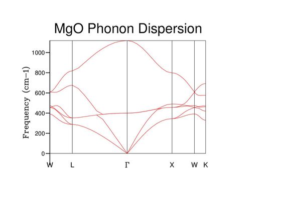  Fig 2: The phonon dispersion curve for the MgO crystal.

The energy dispersion plot (Fig 2) indicates the frequency of vibration (energy) at each k value. Although it resembles a set of continuous curves, it is actually a collection of discrete energy levels so large that they converge to band patterns.

• 
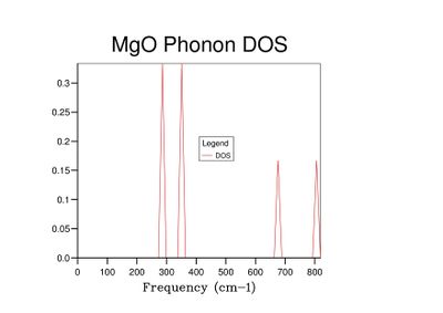  Fig 3: DOS for a 1x1x1 grid.
• 
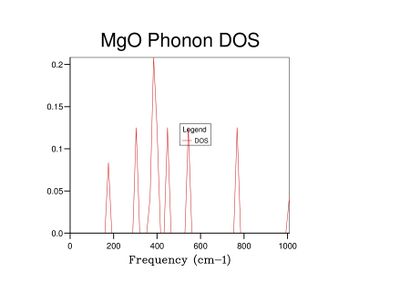  Fig 4: DOS for a 2x2x2 grid.
• 
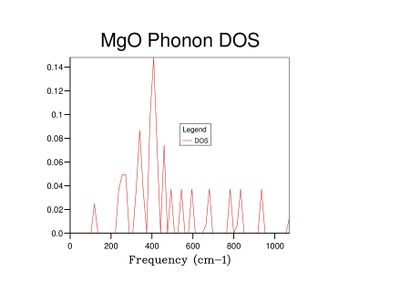  Fig 5: DOS for a 3x3x3 grid.
• 
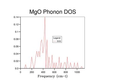  Fig 6: DOS for a 4x4x4 grid.
• 
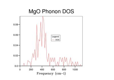  Fig 7: DOS for a 5x5x5 grid.
• 
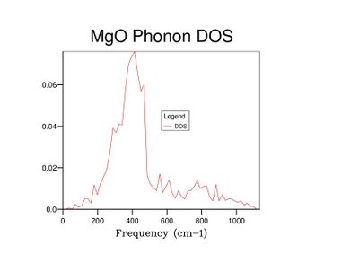  Fig 8: DOS for a 10x10x10 grid.
• 
  Fig 9: DOS for a 15x15x15 grid.
• 
  Fig 10: DOS for a 20x20x20 grid.
• 
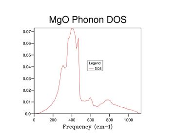  Fig 11: DOS for a 25x25x25 grid.
• 
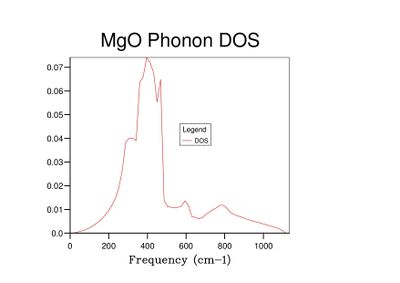  Fig 12: DOS for a 50x50x50 grid.

The Density of States (DOS) is defined as the number of levels between energy E and E + dE, and can be used to group bunches of levels. It is related to the energy dispersion curve in that it is inversely proportional to the slope of E(k) vs. k; the flatter the band, the greater the density of states at a particular energy. The density of states can also be formally related to the energy dispersion E via the following expression:

$DOS(E)=\frac{N}{\pi }\frac{1}{\sqrt{4{\beta }^2-(E-\alpha {)}^2}}$

The grid size defines the number of k-points considered in the calculation. The 1x1x1 DOS (Fig 3) was computed for the k-point corresponding to the symmetry point L, as the frequencies considered in the DOS calculation correspond to those plotted for L in the density of states (Fig 2).

As grid size increases and more k-points are sampled, the number of peaks in the DOS graph increases, and the plot becomes a continuous curve as opposed to a set of discrete peaks. The amount of noise in the curve also decreases with grid size, which is to be expected as more vibrations are sampled and the accuracy of the calculation increases. The minimum grid size that can be used as a reasonable approximation to the density of states is a 25x25x25 grid, which contains an insignificant amount of noise compared to smaller grid sizes.

The size of the reciprocal lattice, which exists in k-space and which is considered in the calculations, is inversely proportional to that of the real-space lattice. The optimal grid size computed for MgO would also be appropriate for a similar oxide such as CaO, as the two structures would be expected to have similar unit cells and lattice parameters. A Zeolite, such as Faujasite, would have a larger real-space lattice than MgO and so would have a smaller reciprocal lattice, thus requiring a smaller grid size. Conversely, a metal such as lithium would have a smaller unit cell, requiring a larger optimum grid size to accurately compute the density of states.

Computing the Free Energy within the Quasi-Harmonic Approximation

Table 1: The variation of free energy with grid size.

Grid Size (n×n×n)	Helmholtz Free Energy (eV)	Deviation from Infinite Grid Value (meV)
1	-40.930301	3.818
2	-40.926609	0.126
3	-40.926432	0.051
4	-40.926450	0.033
5	-40.926463	0.020
10	-40.926480	0.003
15	-40.926482	0.001
20	-40.926483	0.000
25	-40.926483	0.000
50	-40.926483	0.000

• 
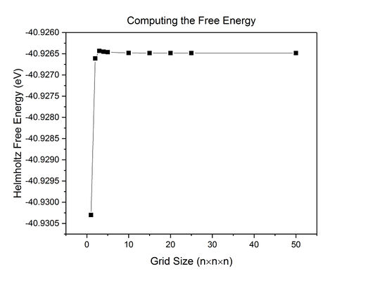  Fig 13: A plot of how Helmholtz free energy varies with grid size.

As the grid size $\to \mathrm{\infty }$, Helmholtz Free Energy A $\to$ -40.926483 (Fig 13).

For a free energy calculation accurate to 1 meV, the minimum grid size that can be used is 2x2x2; this size is also appropriate for calculations accurate to 0.5 meV. A 3x3x3 grid size is the minimum that can be used to obtain a calculation accurate to 0.1 meV.

For all subsequent calculations, a grid size of 25x25x25 was used because, as mentioned above, the density of states contains a negligible amount of noise, and the value for Helmholtz free energy is accurate to at least 0.001 meV.

The Thermal Expansion of MgO

• 
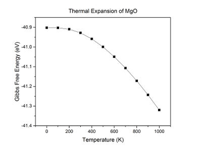  Fig 14: A plot of Gibbs free energy against temperature.
• 
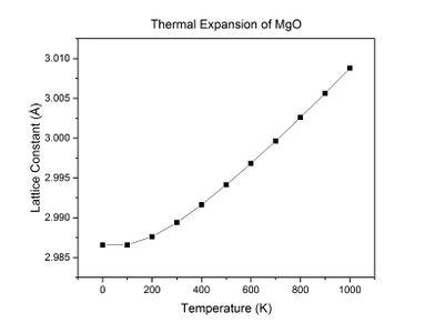  Fig 15: A plot of the lattice constant against temperature.

Throughout the simulation, as temperature increases up to 300 K, Gibbs free energy and the lattice constant do not change significantly. As the temperature is increased above 300 K, Gibbs free energy decreases linearly and the lattice constant increases linearly with temperature. This suggests that the crystal starts to expand at about 200-300 K.

Several approximations are made in the calculation. It is assumed that the behaviour of the ions within the crystal is purely harmonic, and that the free energy is minimised. The force field used excludes the shells of the ions and assumes a short-range, Buckingham repulsive potential operates between the ions. Also, covalent interactions between ions are neglected.

The physical origin of thermal expansion can be explained using an anharmonic potential. At 0 K, the atoms in the crystal have a zero-point energy which causes them to oscillate in a coupled, parabolic fashion. As the temperature increases, the average energy of the ions increases by $k_{B}T$. This causes the amplitude of oscillation and thus equilibrium interatomic separation to increase, as the vibrations of the ions become more anharmonic. The free energy decreases upon expansion because of the thermodynamic relationship between free energy and temperature: $A=U-TS$. As temperature increases and the second term becomes larger, the free energy naturally decreases. It also decreases as a result of a lowering of the phonon frequencies.

As the temperature approaches the melting point of MgO, the phonon modes would be expected to be less representative of the actual motions of the ions. This is because as temperature increases, the motions of the ions become more anharmonic. However, as the temperature range simulated in this experiment is well below the melting point (lit. 3098 K), anharmonic perturbations can be assumed to be negligible.

In a diatomic molecule with an exactly harmonic potential, the bond length would not be expected to increase with temperature because the harmonic model assumes an equilibrium bond length that is independent of temperature. The quasi-harmonic approximation overcomes this by assuming that bond vibrations follow the harmonic model, but that phonon frequencies are volume-dependent. Changes in phonon frequencies result in a change in the free energy, from which the equilibrium volume can be derived.

Molecular Dynamics

• 
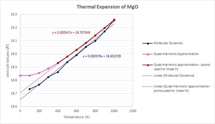  Fig 16: Plots of the thermal expansions of each simulation.

Table 2: A summary of the calculated thermal expansion coefficients.

Simulation	α (10-5 K-1)	Error (%) lit. 3.11×10-5 K-1
Quasi-Harmonic Approximation	2.89	7.10
Molecular Dynamics	3.09	0.63

At lower temperatures, the unit cell volumes predicted by the molecular dynamics simulations are significantly lower than those predicted by the quasi-harmonic approach (Fig 16). However, as temperature increases (noticeably beyond 500 K), the two trends begin to converge and the volumes measured at 1000 K are almost identical.

The value of the thermal expansion coefficient calculated from the molecular dynamics simulations is incredibly close to the experimentally determined literature value, which was carried out at a pressure of 0 GPa and a temperature of approximately 298 K. The value calculated from the linear portion of the quasi-harmonic plot deviates more from the expected value. The results from this suggest that molecular dynamics is a more accurate method to simulate the thermal expansion of a system. The fact that the literature value was measured only at room temperature must be taken into account, however, since this could affect the ability to make a meaningful comparison with the simulation data, which was obtained for a wider temperature range

The data obtained from the quasi-harmonic approximation show an initial plateau in volume, whereas those from the molecular dynamics simulations do not. This is because the former, unlike the latter, takes zero-point energy into account. This may suggest that molecular dynamics is less accurate at lower temperatures.

For molecular dynamics to be able to perform a reliable calculation, a larger cell size must be used. The 32 unit cells considered in the computation would be expected to only contain a small number of k-points; the small sample size used during the calculation would have affected the accuracy of the results. The grid size of 25x25x25 used for the quasi-harmonic calculations would certainly give far more accurate results, but in reality is likely to require too much computational power to be feasible. A 15x15x15 grid has been shown to give a free energy value accurate to 0.001 meV (Table 1) and the calculated DOS is a reasonable approximation (Fig 9). However, this is still likely to require a large amount of computational power.

At higher temperatures, particularly those beyond the melting point of MgO, the quasi-harmonic approximation would eventually fail, underestimating the cell volume. This is because anharmonic phonon interactions, which the quasi-harmonic approximation does not consider, begin to dominate.. At lower temperatures, these anharmonic interactions become low enough to be negligible, resulting in more accurate simulations. Additionally, the quasi-harmonic approximation also fails to consider the possibility of bond dissociation, which molecular dynamics takes into account. Therefore molecular dynamics is likely to yield more accurate cell volumes at very high temperatures, and also show phase transitions, possibly through changes in the gradient of temperature vs. volume.

Conclusion

In this experiment, the thermal expansion of an MgO crystal was simulated at a temperature range of 0-1000 K using GULP software, and the thermal expansion coefficient was calculated. The simulations were performed using both a quasi-harmonic approximation and a molecular dynamics approach, and the results were compared to determine the validity of each approach.

It was found that the thermal expansion coefficient calculated from the molecular dynamics approach was in good agreement with the literature value, whereas that from the quasi-harmonic simulations noticeably deviated. The results from these simulations suggest that molecular dynamics is a more appropriate approach to use at higher temperatures, since it considers deviations from the harmonic approximation and the possibility of bond dissociation. However, the small sample size of 32 MgO cell units used in the calculations is likely to compromise the accuracy of the results to some extent.

For the temperature range used in the simulation, the quasi-harmonic approximation is likely to be more appropriate because the 25x25x25 grid size allows a much larger sample of vibrational frequencies to be considered without requiring an unreasonably large amount of computational power. Additionally, as the temperature range considered is generally low, anharmonic phonon interactions are negligible, so the harmonic oscillator is a reasonable approximation to the vibrational motions in the crystal.

In future experiments, it would be interesting to compare each approach at a higher temperature range, particularly around the melting point of MgO (for example 3000-4000 K), to visualise how each trend would behave and how accurately they would reflect the real-life behaviour of the crystal.

References

- ↑ 1.0 1.1 1.2 W. Cochran, in The Dynamics of Atoms in Crystals, ed. B. R. Coles, Edward Arnold Publishers Limited, London, 1973, ch. 8, pp. 101-111.
- ↑ M.T. Dove, in Introduction to Lattice Dynamics, Cambridge University Press, Cambridge, 1993, ch. 12, pp. 179-194.
- ↑ P. Atkins and J. de Paula, in Atkins' Physical Chemistry, Oxford University Press, Oxford, 9th edn, 2010, ch. 15, pp. 564-591.
- ↑ 4.0 4.1 R. Hoffmann, Angew. Chem. Int. Ed. Engl., 1987, 26, 846-878.
- ↑ A. P. Sutton, in Electronic Structure of Materials, Oxford University Press, Oxford, 1993, ch. 4, pp. 89-92.
- ↑ R. Turton, in The Physics of Solids, Oxford University Press, Oxford, 2002, ch. 7, pp 187-189.
- ↑ W.M. Haynes, CRC Handbook of Chemistry and Physics, CRC Press Inc., Boca Raton, FL, 91st edn, 2010-2011, pp. 4-74
- ↑ M.T. Dove, in Introduction to Lattice Dynamics, Cambridge University Press, Cambridge, 1993, ch. 2, pp. 18-35.
- ↑ 9.0 9.1 A.Chopelas, Phys Chem Minerals, 1990, 17, 142-148.