Monte-Carlo simulations of a 2D Ising Model

TASK1

Show that the lowest possible energy for the Ising model is $E = - D N J$ , where $D$ is the number of dimensions and $N$ is the total number of spins. What is the multiplicity of this state? Calculate its entropy.

The lowest possible energy state is when all of the spins are pointing at the same direction i.e. all up (all s_i=+1) or all down (all s_i=-1). At this state s_i*s_j will be 1. Each spin has 2D neighbours. E = -0.5*J*N*2D = -DNJ. Multiplicity is 2 because there are two possible configurations of the lowest possible energy state, all up or all down. S = K_BlnΩ = K_B*ln2 = 9.565*10^-24 JK^-1

TASK2

Imagine that the system is in the lowest energy configuration. To move to a different state, one of the spins must spontaneously change direction ("flip"). What is the change in energy if this happens ( $D = 3, N = 1000$ )? How much entropy does the system gain by doing so?

In a 3D lattice, each spin has 6 neighbours. When flipping a spin, s_i*s_j will change to -1. The contribution to energy of this spin will change from +6J to -6J. So the change in energy is 12J. The number of possible configurations of this state is now 2*1000!/999!=2000 (times by two because original state can be all up or all down). The new entropy is K_B*ln2000=1.049*10^-22 JK^-1 and the increase in entropy is 9.533*10^-23 JK^-1.

TASK3

Calculate the magnetisation of the 1D and 2D lattices in figure 1. What magnetisation would you expect to observe for an Ising lattice with $D = 3, N = 1000$ at absolute zero?

M_1D=+1. M_2D=+1. At absolute zero, the energetic driving force dominates and all the spins will be parallel. M_3D=±1000 at T=0K.

TASK4

complete the functions energy() and magnetisation(), which should return the energy of the lattice and the total magnetisation, respectively. In the energy() function you may assume that $J = 1.0$ at all times (in fact, we are working in reduced units in which $J = k_{B}$ , but there will be more information about this in later sections). Do not worry about the efficiency of the code at the moment — we will address the speed in a later part of the experiment.

   def energy(self):
       "Return the total energy of the current lattice configuration."
       energy=0
       for i in range(len(self.lattice)):
           for j in range(len(self.lattice)):
               s=self.lattice[i,j]
               neighbour=self.lattice[(i+1)%self.n_rows,j]+self.lattice[i,(j+1)%self.n_cols]+self.lattice[(i-1)%self.n_rows,j]+self.lattice[i,(j-1)%self.n_cols]
               energy += -neighbour*s
       
       return energy/2

   def magnetisation(self):
       "Return the total magnetisation of the current lattice configuration."
       magnetisation=np.sum(self.lattice)
       return magnetisation

TASK5

Run the ILcheck.py script from the IPython Qt console using the command

%run ILcheck.py

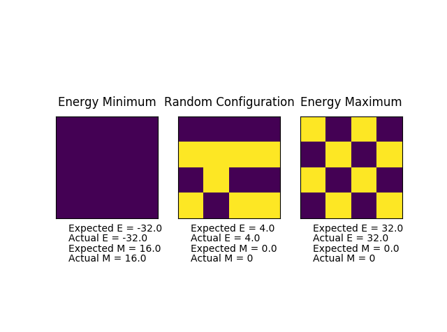
The displayed window has a series of control buttons in the bottom left, one of which will allow you to export the figure as a PNG image. Save an image of the ILcheck.py output, and include it in your report.

**Figure 1.** Test result from ILcheck.py. Expected values matches with actual values showing the code is correct.

TASK6

How many configurations are available to a system with 100 spins? To evaluate these expressions, we have to calculate the energy and magnetisation for each of these configurations, then perform the sum. Let's be very, very, generous, and say that we can analyse $1 \times 1 0^{9}$ configurations per second with our computer. How long will it take to evaluate a single value of ${⟨ M ⟩}_{T}$ ?

For a system with 100 spins, there are 2¹⁰⁰=1.268*10³⁰ configurations. Time taken is 1.268*10³⁰/10⁹ = 1.268*10²¹ seconds.

TASK7

Implement a single cycle of the above algorithm in the montecarlocycle(T) function. This function should return the energy of your lattice and the magnetisation at the end of the cycle. You may assume that the energy returned by your energy() function is in units of $k_{B}$ ! Complete the statistics() function. This should return the following quantities whenever it is called: $< E >, < E^{2} >, < M >, < M^{2} >$ , and the number of Monte Carlo steps that have elapsed.

   def montecarlostep(self, T):
       # complete this function so that it performs a single Monte Carlo step
       E0 = self.energy()
       #the following two lines will select the coordinates of the random spin for you
       random_i = np.random.choice(range(0, self.n_rows))
       random_j = np.random.choice(range(0, self.n_cols))
       if self.lattice[random_i][random_j]==1:
           self.lattice[random_i][random_j]=-1
       else:
           self.lattice[random_i][random_j]=1
       E1=self.energy()
       dE=E1-E0
       if dE<=0:
           self.lattice[random_i][random_j] = 1*self.lattice[random_i][random_j]
       elif dE>0:
           R=np.random.random()
           if R<= math.exp(-dE/T):
               self.lattice[random_i][random_j]=1*self.lattice[random_i][random_j]
           else:
               self.lattice[random_i][random_j]=-1*self.lattice[random_i][random_j]
       self.n_cycles+=1
       self.E+=self.energy()
       self.E2+=self.energy()**2
       self.M+=self.magnetisation()
       self.M2+=self.magnetisation()**2        
       return self.energy(), self.magnetisation()

   def statistics(self):
       # complete this function so that it calculates the correct values for the averages of E, E*E (E2), M, M*M (M2), and returns them
       return self.E/self.n_cycles, self.E2/self.n_cycles, self.M/self.n_cycles, self.M2/self.n_cycles, self.n_cycles

TASK8

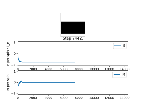
If $T < T_{C}$ , do you expect a spontaneous magnetisation (i.e. do you expect $⟨ M ⟩ \neq 0$ )? When the state of the simulation appears to stop changing (when you have reached an equilibrium state), use the controls to export the output to PNG and attach this to your report. You should also include the output from your statistics() function.

When T<T_C, energetic driving force dominates so spins tend to become parallel and energy will tend to the lowest possible value. A spontaneous magnetisation is expected. <M> is expected to be non-zero.

TASK9

Use the script ILtimetrial.py to record how long your current version of IsingLattice.py takes to perform 2000 Monte Carlo steps. This will vary, depending on what else the computer happens to be doing, so perform repeats and report the error in your average!

Number of run	Time taken/s
1	8.492
2	8.525
3	8.566
4	8.677
5	8.581
6	8.431
7	8.458
8	8.597
9	8.660
10	8.692

The average value of times taken is calculated to be 8.568±0.295 seconds.

TASK10

Look at the documentation for the NumPy sum function. You should be able to modify your magnetisation() function so that it uses this to evaluate M. The energy is a little trickier. Familiarise yourself with the NumPy roll and multiply functions, and use these to replace your energy double loop (you will need to call roll and multiply twice!).

   def energy(self):
       "Return the total energy of the current lattice configuration."
       energy=0
       energy=-np.sum(np.multiply(self.lattice,np.roll(self.lattice, 1, axis=1))+np.multiply(self.lattice,np.roll(self.lattice, 1, axis=0)))  
       return energy

   def magnetisation(self):
       "Return the total magnetisation of the current lattice configuration."
       magnetisation=np.sum(self.lattice)
       return magnetisation

TASK11

Use the script ILtimetrial.py to record how long your new version of IsingLattice.py takes to perform 2000 Monte Carlo steps. This will vary, depending on what else the computer happens to be doing, so perform repeats and report the error in your average!

Number of run	Time taken/s
1	0.390
2	0.394
3	0.389
4	0.393
5	0.394
6	0.389
7	0.390
8	0.393
9	0.387
10	0.393

The average value of times taken is calculated to be 0.391±0.047 seconds, which is much faster than the old version.

TASK12

The script ILfinalframe.py runs for a given number of cycles at a given temperature, then plots a depiction of the final lattice state as well as graphs of the energy and magnetisation as a function of cycle number. This is much quicker than animating every frame! Experiment with different temperature and lattice sizes. How many cycles are typically needed for the system to go from its random starting position to the equilibrium state? Modify your statistics() and montecarlostep() functions so that the first N cycles of the simulation are ignored when calculating the averages. You should state in your report what period you chose to ignore, and include graphs from ILfinalframe.py to illustrate your motivation in choosing this figure.

**Figure 4.** Energy and magnetisation per spin vs temperature of a 8x8 lattice at 1K. It takes around 500 cycles for a 8x8 lattice to reach equilibrium at 1K.

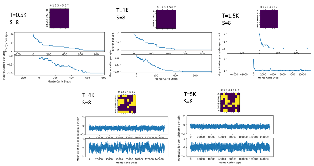
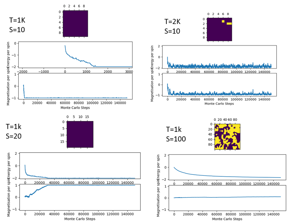
It takes more cylces for a larger lattice to reach equilibrium. For a 20x20 lattice, around 3000 cycles are needed, which is 7.5 times of the number of spins in the system. A compromise has to be made between less simulation time and more accurate simulation. So instead of using a constant number as N, 200 times of number of spin is chosen as the number of cycles to ignore before the system reaches equilibrium.

   def montecarlostep(self, T):
       # complete this function so that it performs a single Monte Carlo step
       E0 = self.energy()
       #the following two lines will select the coordinates of the random spin for you
       random_i = np.random.choice(range(0, self.n_rows))
       random_j = np.random.choice(range(0, self.n_cols))
       if self.lattice[random_i][random_j]==1:
           self.lattice[random_i][random_j]=-1
       else:
           self.lattice[random_i][random_j]=1
       E1=self.energy()
       dE=E1-E0
       if dE<=0:
           self.lattice[random_i][random_j] = 1*self.lattice[random_i][random_j]
       elif dE>0:
           R=np.random.random()
           if R<= math.exp(-dE/T):
               self.lattice[random_i][random_j]=1*self.lattice[random_i][random_j]
           else:
               self.lattice[random_i][random_j]=-1*self.lattice[random_i][random_j]
       self.n_cycles+=1
       
       if self.n_cycles>self.n_rows*self.n_cols*200:
           self.E+=self.energy()
           self.E2+=self.energy()**2
           self.M+=self.magnetisation()
           self.M2+=self.magnetisation()**2
       else:
           pass
       
       return self.energy(), self.magnetisation()

   def statistics(self):
       # complete this function so that it calculates the correct values for the averages of E, E*E (E2), M, M*M (M2), and returns them
       return self.E/(self.n_cycles-self.n_rows*self.n_cols*200), self.E2/(self.n_cycles-self.n_rows*self.n_cols*200), self.M/(self.n_cycles-self.n_rows*self.n_cols*200), self.M2/(self.n_cycles-self.n_rows*self.n_cols*200), self.n_cycles-self.n_rows*self.n_cols*200

TASK13

Use ILtemperaturerange.py to plot the average energy and magnetisation for each temperature, with error bars, for an $8 \times 8$ lattice. Use your initution and results from the script ILfinalframe.py to estimate how many cycles each simulation should be. The temperature range 0.25 to 5.0 is sufficient. Use as many temperature points as you feel necessary to illustrate the trend, but do not use a temperature spacing larger than 0.5. T NumPy function savetxt() stores your array of output data on disk — you will need it later. Save the file as 8x8.dat so that you know which lattice size it came from.

100000 runtime was used and simulation was carried out from 0.3K to 5.0K with interval of 0.1K. 3 repeats were carried out.

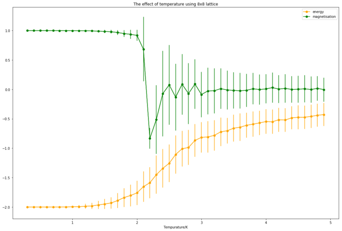
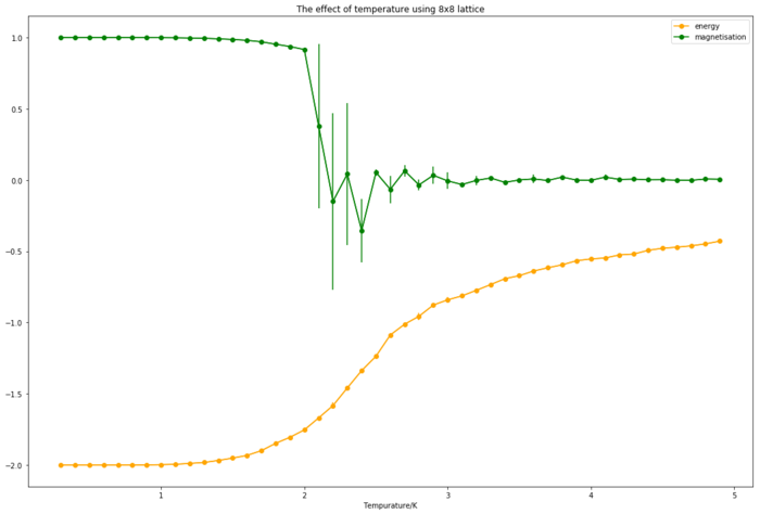
As it can be seen from figure 7 that energy and magnetisation fluctuate more at higher temperature because of greater probability of spin flipping. 3 repeats were carried out because there is no guarantee that every configuration will reach equilibrium. As it can be seen from figure 8 that there is no significant difference between energy of each configuration but magnetisation varies significantly during phase transition.

TASK14

Repeat the final task of the previous section for the following lattice sizes: 2x2, 4x4, 8x8, 16x16, 32x32. Make sure that you name each datafile that your produce after the corresponding lattice size! Write a Python script to make a plot showing the energy per spin versus temperature for each of your lattice sizes. Hint: the NumPy loadtxt function is the reverse of the savetxt function, and can be used to read your previously saved files into the script. Repeat this for the magnetisation. As before, use the plot controls to save your a PNG image of your plot and attach this to the report. How big a lattice do you think is big enough to capture the long range fluctuations?

100000 runtime was used for 2x2, 4x4, 8x8 lattice. 300000 runtime was used for 16x16 lattice. 500000 runtime was used for 32x32 lattice.

def plot_e_m(x):

   data= np.loadtxt(x)
   l=int(x.split('x')[0])
   n=l**2
   t=data[:,0]
   e=data[:,1]/n
   e2=data[:,2]/n**2
   m=data[:,3]/n
   m2=data[:,4]/n**2
   eerr=(e2-e**2)**0.5
   merr=(m2-m**2)**0.5
   ns=str(l)
   figure(figsize=[18,12])
   errorbar(t, e,  yerr=eerr,color='orange')
   errorbar(t, m,  yerr=merr,color='green')
   plot(t, e, color='orange',marker='o',label='energy')
   plot(t,m,color='green',marker='o',label='magnetisation')
   xlabel('Tempurature/K')
   legend()
   title('The effect of temperature using '+ns+'x'+ns+' lattice')
   show()
   return

plot_e_m('2x2_new.dat')

for averaging 3 repeats:

def enermagne(x,y,z):

   datax = np.loadtxt(x)
   datay = np.loadtxt(y)
   dataz = np.loadtxt(z)
   l=int(x.split('x')[0])
   n=l**2
   t=datax[:,0]
   e=(datax[:,1]+datay[:,1]+dataz[:,1])/(n*3)
   m=(datax[:,3]+datay[:,3]+dataz[:,3])/(n*3)
   E=[datax[:,1]/n,datay[:,1]/n,dataz[:,1]/n]
   M=[datax[:,3]/n,datay[:,3]/n,dataz[:,3]/n]
   eerr=np.std(E, axis = 0)
   merr=np.std(M, axis = 0)
   figure(figsize=[18,12])
   errorbar(t, e,  yerr=eerr,color='orange')
   errorbar(t, m,  yerr=merr,color='green')
   plot(t, e, color='orange',marker='o',label='energy')
   plot(t,m,color='green',marker='o',label='magnetisation')
   xlabel('Tempurature/K')
   legend()
   ns=str(l)
   title('The effect of temperature using '+ns+'x'+ns+' lattice')
   show()
   return

enermagne('32x32_new.dat','32x32_newone.dat','32x32_repeat1.dat')

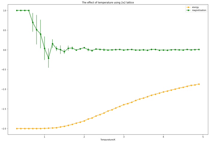
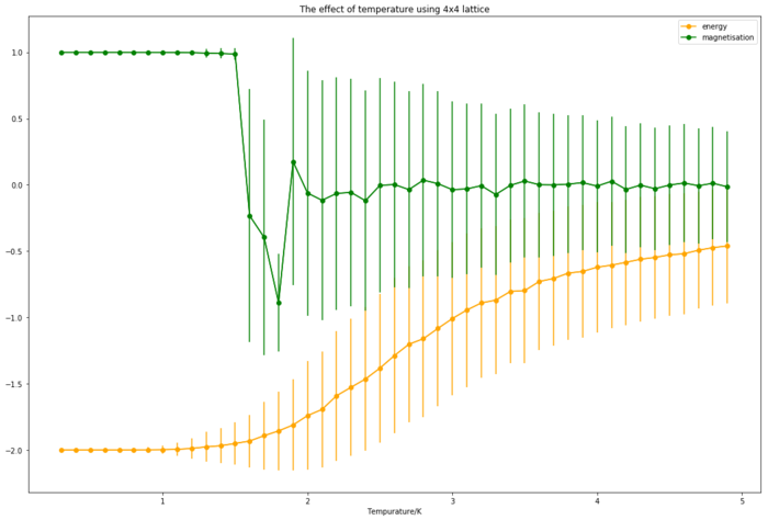
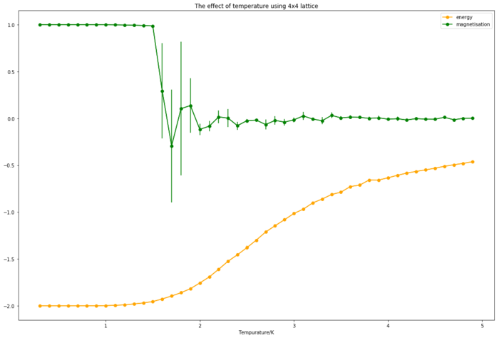
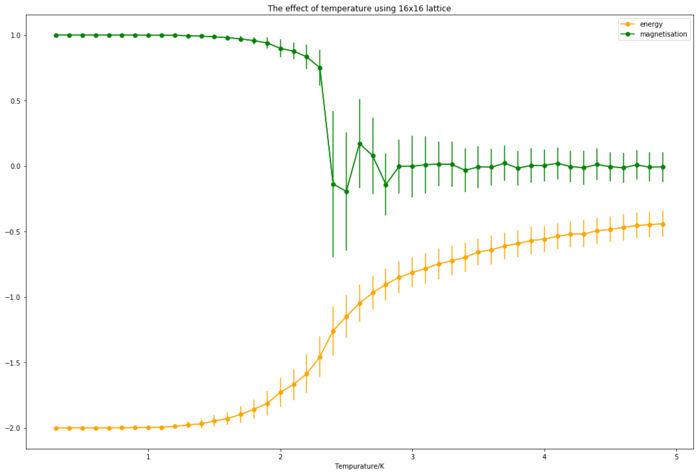
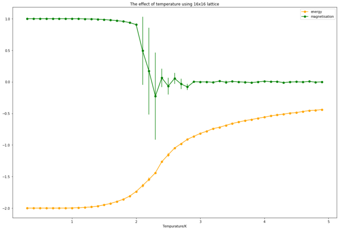
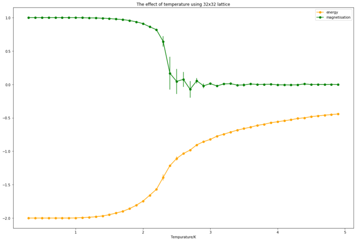
Energy and magnetisation fluctuate more at higher temperature. There is no significant difference between energy of each configuration but magnetisation varies significantly during phase transition. 2x2 and 4x4 are too small for a good simulation because they both have large error bars showing significant fluctuations at high temperature. 16x16 will be a good lattice size to use in order to capture a long range fluctuation considering less simulation time is wanted.

TASK15

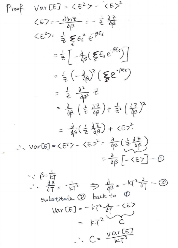
TASK: By definition,

$C = \frac{\partial ⟨ E ⟩}{\partial T}$

From this, show that

$C = \frac{V a r [E]}{k_{B} T^{2}}$

(Where $V a r [E]$ is the variance in $E$ .)

TASK16

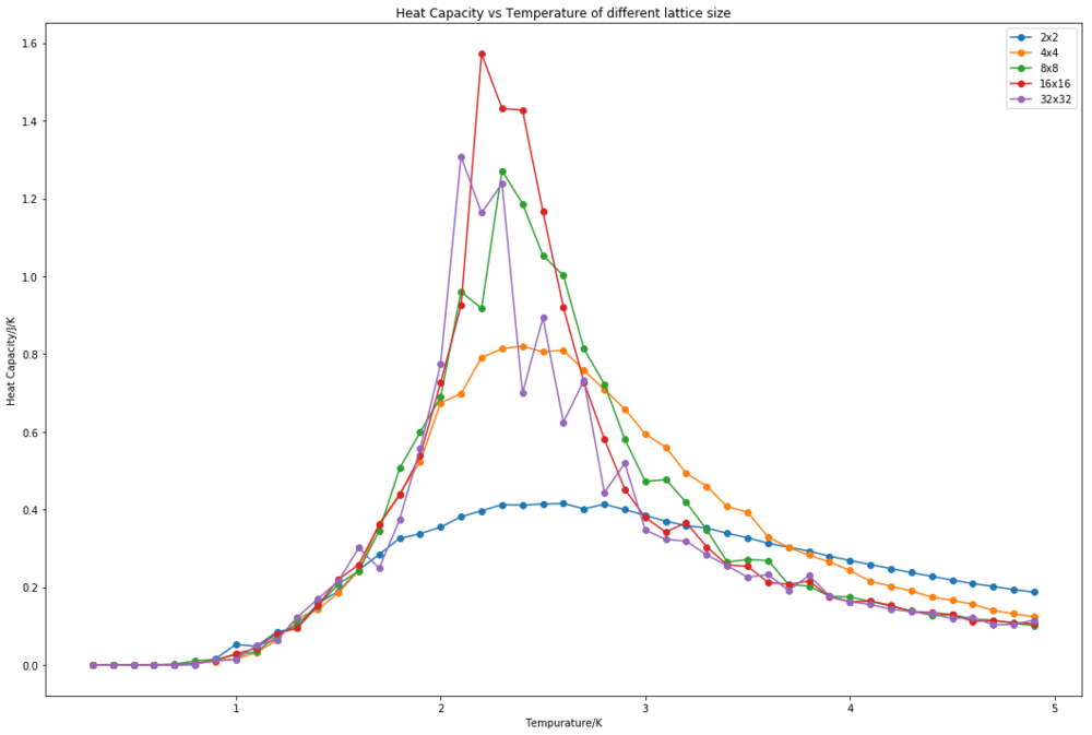
Write a Python script to make a plot showing the heat capacity versus temperature for each of your lattice sizes from the previous section. You may need to do some research to recall the connection between the variance of a variable, $V a r [X]$ , the mean of its square $⟨ X^{2} ⟩$ , and its squared mean ${⟨ X ⟩}^{2}$ . You may find that the data around the peak is very noisy — this is normal, and is a result of being in the critical region. As before, use the plot controls to save your a PNG image of your plot and attach this to the report.

def heatcapa(x):

   data=np.loadtxt(x)
   l=int(x.split('x')[0])
   n=l**2
   t=data[:,0]
   e=data[:,1]
   e2=data[:,2]
   c=(e2-(e**2))/((t**2)*n)
   ns=str(l)
   figure(figsize=[18,12])
   plot(t, c, color='orange',marker='o')
   xlabel('Tempurature/K')
   ylabel('Heat Capacity/J/K')
   title('Heat Capacity versus Temperature of '+ns+'x'+ns+' Lattice')
   show()
   return

heatcapa('32x32_new.dat')

TASK17

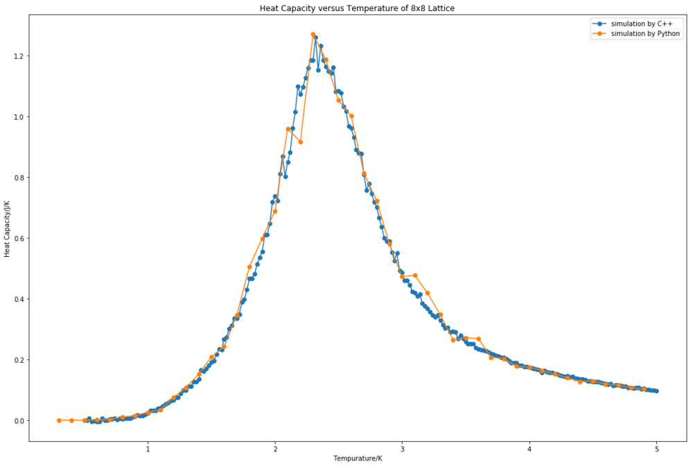
A C++ program has been used to run some much longer simulations than would be possible on the college computers in Python. You can view its source code here if you are interested. Each file contains six columns: $T, E, E^{2}, M, M^{2}, C$ (the final five quantities are per spin), and you can read them with the NumPy loadtxt function as before. For each lattice size, plot the C++ data against your data. For one lattice size, save a PNG of this comparison and add it to your report — add a legend to the graph to label which is which. To do this, you will need to pass the label="..." keyword to the plot function, then call the legend() function of the axis object (documentation here).

TASK18

write a script to read the data from a particular file, and plot C vs T, as well as a fitted polynomial. Try changing the degree of the polynomial to improve the fit — in general, it might be difficult to get a good fit! Attach a PNG of an example fit to your report.

def polyfit(x):

   data = np.loadtxt(x) #assume data is now a 2D array containing two columns, T and C
   T = data[:,0] #get the first column
   C = data[:,5] # get the second column
   l=int(x.split('x')[0])
   n=l**2
   fit = np.polyfit(T, C, 37) # fit a third order polynomial
   T_min = np.min(T)
   T_max = np.max(T)
   T_range = np.linspace(T_min, T_max, 1000) #generate 1000 evenly spaced points between T_min and T_max
   fitted_C_values = np.polyval(fit, T_range) # use the fit object to generate the corresponding values of C
   figure(figsize=[18,12])
   plot(T, C, marker='o',label='data')
   plot(T_range, fitted_C_values, marker='o', label='polynomial fitting')
   ns=str(l)
   xlabel('Tempurature/K')
   ylabel('Heat Capacity/J/K')
   legend()
   title('polynomial fitting versus simulation data of '+ns+'x'+ns+' Lattice')
   show()

polyfit('16x16_new.dat')

TASK19

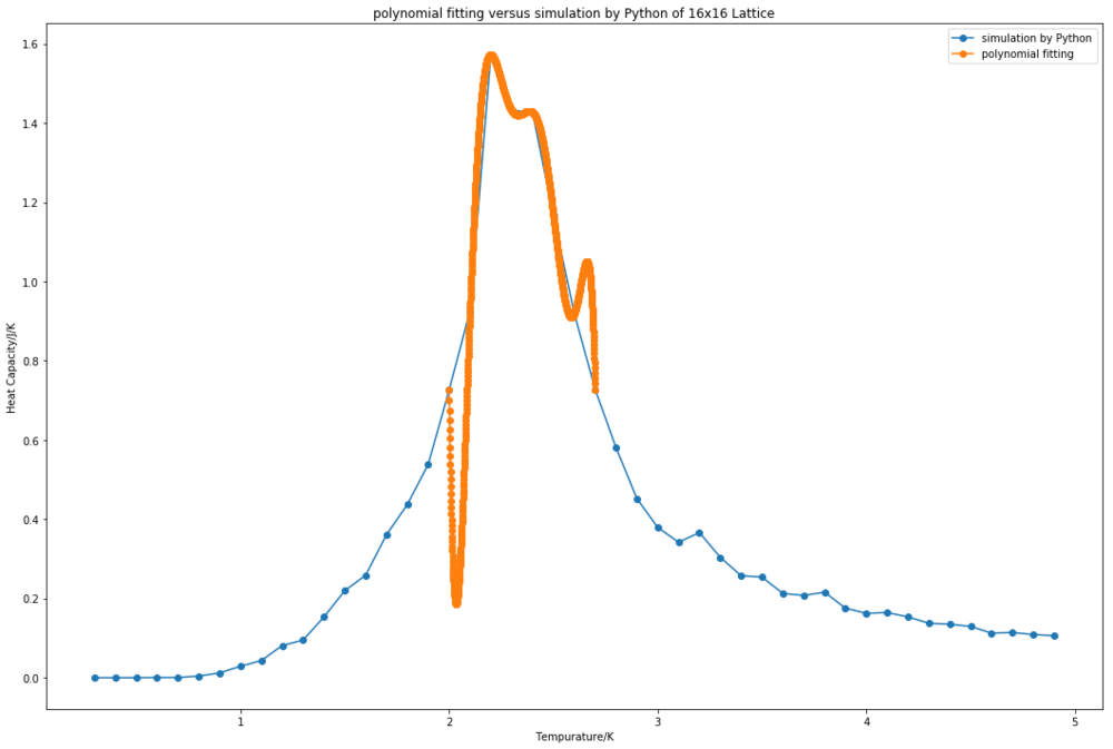
Modify your script from the previous section. You should still plot the whole temperature range, but fit the polynomial only to the peak of the heat capacity! You should find it easier to get a good fit when restricted to this region.

def ownpolyfit(x):

   data = np.loadtxt(x)
   l=int(x.split('x')[0])    
   T = data[:,0] #get the first column
   C = (data[:,2]-(data[:,1])**2)/(T**2*(l**2)) # get the second column
   Tmin = 2 #for example
   Tmax = 2.8 #for example
   selection = np.logical_and(T > Tmin, T < Tmax) #choose only those rows where both conditions are true
   peak_T_values = T[selection]
   peak_C_values = C[selection]
   fit = np.polyfit(peak_T_values, peak_C_values, 7) # fit a third order polynomial
   T_min = np.min(peak_T_values)
   T_max = np.max(peak_T_values)
   T_range = np.linspace(T_min, T_max, 1000) #generate 1000 evenly spaced points between T_min and T_max
   fitted_C_values = np.polyval(fit, T_range) # use the fit object to generate the corresponding values of C    
   ns=str(l)
   figure(figsize=[18,12])
   plot(T, C, marker='o',label='simulation by Python')
   plot(T_range, fitted_C_values, marker='o', label='polynomial fitting')
   xlabel('Tempurature/K')
   ylabel('Heat Capacity/J/K')
   legend()
   title('polynomial fitting versus simulation by Python of '+ns+'x'+ns+' Lattice')
   show()    
   Cmax = np.max(fitted_C_values)
   Tmax = T_range[fitted_C_values == Cmax]
   return (Cmax, Tmax)

ownpolyfit("16x16_new.dat")

TASK20

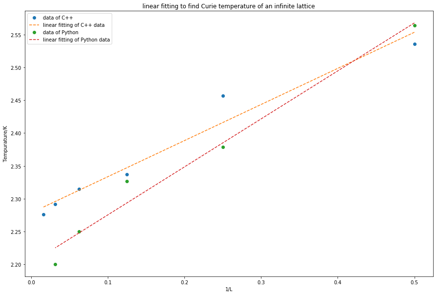
find the temperature at which the maximum in C occurs for each datafile that you were given. Make a text file containing two colums: the lattice side length (2,4,8, etc.), and the temperature at which C is a maximum. This is your estimate of $T_{C}$ for that side length. Make a plot that uses the scaling relation given above to determine $T_{C, \infty}$ . By doing a little research online, you should be able to find the theoretical exact Curie temperature for the infinite 2D Ising lattice. How does your value compare to this? Are you surprised by how good/bad the agreement is? Attach a PNG of this final graph to your report, and discuss briefly what you think the major sources of error are in your estimate.

According to equation T_C,L=A/L+T_C,∞, T_C,L was plotted against 1/L. T_C,∞, the Curie temperature for the infinite 2D Ising lattice, is the intercept with y axis. T_C,∞ found using the Python data is 2.202K and literature value found is 2.269K^[1], which is closer to the value found using C++ data (2.279K). There is 3% difference between the experimental value and theoretical value. The major source of error is that temperature interval of 0.1K is not small enough to produce an accurate simulation. 0.1K was chosen due to time limitation but the maximum heat capacity may lay between the sampling temperatures. Data by C++ simulation gives much closer result so more sampling temperature should be used. Also simulations should be carried out for more different lattice sizes to give a better linear fitting.

**Figure 21.** Linear fitting to find Curie temperature of an infinite lattice.

REFERENCE

[1] L. Onsager, Phys. Rev., 1944, 65, 117.