
Rep:Mod:jgh002
Julia Gonzalez Holguera Computational Laboratory Module 2
Molecular modelling is a computer based technique which allows, upon theoretical grounds, to optimise structures of molecules and determinine some of their properties. Different computational methods have been developed and are now widely used by chemists to rationalize and predict structure and reactivity of molecules.
This module will aim to introduce us to some computational methods, focusing on showing how after a geometry optimisation and frequency analysis, some molecular properties can be predicted computationally.
Part 1: Structural and Molecular Orbital analysis of BH3 and TlBr3
The first part of this module will aim familiarize ourselves with computational methods. This will be done studying two simple molecules, BH3 and TlBr3. BH3 will be studied first. It's vibrational spectrum as well as its molecular orbitals (MOs) will be determined and analysed. The (MOs) will be compared to those obtained from a simple LCAO approach. The vibrational frequencies of TlBr3 and the method used to determine these will be briefly discussed.
Analysis of BH3
Optimisation
The optimisation of the geometry of the molecule was the first step to the study of the molecule. This was performed using the
opt b3lyp/3-21g geom=connectivity

method in the Gaussian. The optimisation proceeds by calculating the electron densities and energies of the molecule for given positions of the nuclei

and repeating the calculations until the values converge and a lowest energy structure is found.
The optimisation is reported in Figure 1, and shows the energies for the different structures, which converge at the fourth geometry.

By looking at the optimised geometry, it is found that the molecule is characterised by an H-B-H angle of 120° and a bond length of 1.19 Å. The bond angle reflects the three-fold symmetry of the planar molecule, and the bond length is in good agreement with literature[1]. This therefore shows that despite using the low accuracy basis set 3-21G, which completed the optimisation after only four iterations, the results of the optimisation for the simple BH3 molecule are none-the-less in good agreement with literature.
A summary of the informations which have been calculated by the program can be found in Table 1

. The point group, the dipole moment and the energy of the molecule are key informations displayed in the table. The RMS Gradient Norm <0.001 serves as an indication that the optimisation has completed. This is confirmed by looking directly at the Gaussian output file which states that a stationary point was found. Looking at the frequencies will ensure that the structure obtained actually corresponds to a minimum (and not to a transition state).
Vibrational frequencies
The vibrational frequencies of BH3 were calculated on the optimsied structure using the following method/basis set:
freq b3lyp/3-21g geom=connectivity pop=(full,nbo)
The calculation can be accessed here [Gaussian SCAN result :DOI:10042/to-12935 ], and the main data is reported in Table 2.
However, before discussing the main vibrations it is important to check the signs of the frequencies computed. Indeed, as the frequencies are the second derivative of the potential energy surface, looking at the sign of the vibrations allows to check whether the structure is indeed a minimum in energy. If the frequencies are all positive, then we have a minimum. If one of them is negative we have a transition state, and if any more are negative then the optimisation has essentially failed. In the present calculation all the frequencies are positive, it can therefore be assumed that the optimisation has converged to a minimum.
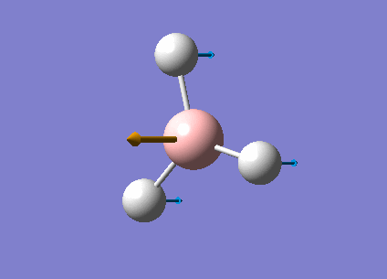
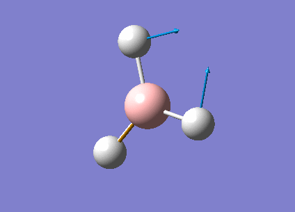
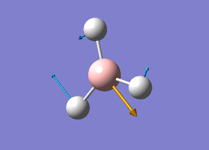
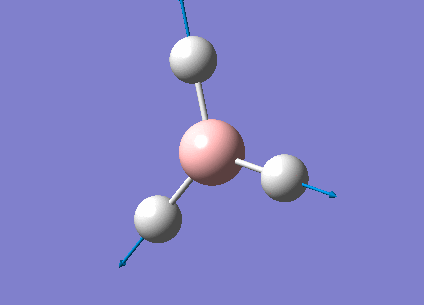
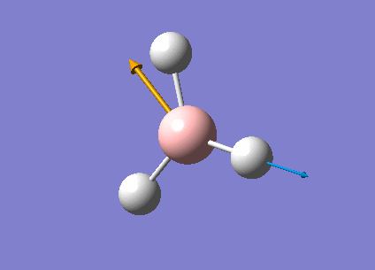
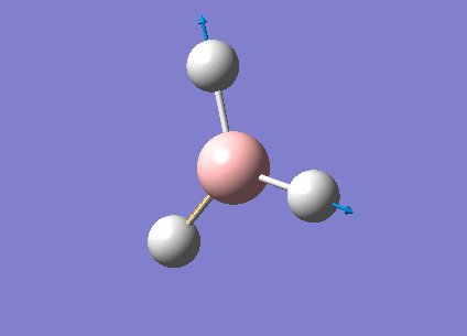
| Form of the vibrations | Frequency (cm-1) | Intensity | Symmetry D3h Point Group | Representation | Diagram | |
|---|---|---|---|---|---|---|
| 1 | The three hydrogens atoms are moving concertedly in the opposite direction to the boron atom.
The displacement is greater for the hydrogen atoms than for the boron atoms because the former have a greater reduced mass. |
1144.15 | 92.8665 | A2" | Media:Vibration1jgh.gif |  |
| 2 | Scissor bend of two hydrogen atoms and little displacement of the remaining hydrogen and the
boron atoms. |
1203.64 | 12.3148 | E' | Media:Vibration2jgh.gif |  |
| 3 | Scissor bend of Hydrogens 2 & 3 with movement in the same direction and displacement of atom 3 in opposite direction. | 1203.64 | 12.3173 | E' | Media:Vibration3jgh.gif |  |
| 4 | Fully symmetrical B-H stretches | 2598.42 | 0.0000 | A1' | Media:Vibration4jgh.gif |  |
| 5 | Asymmetric stretch of B-H 1 & 2 with small displacement of the boron atom. | 2737.44 | 103.7400 | E' | Media:Vibration5jgh.gif |  |
| 6 | B-H stretches. In phase for hydrogen 1 & 2 and out-of-phase for hydrogen 3. | 2737.44 | 103.7333 | E' | Media:Vibration6jgh.gif |  |

The data was represented as an IR spectrum that is reported in Figure 3.
It can be seen that, while the molecule has six vibrations, only 5 of them appear on the spectrum. This is because even if Vibration 4 exists, it is not IR active because it is fully symetrical. In other words, the vibration does not give rise to a change in dipole moment, which explains why it is not IR active.
It is also worth noting that Vibrations 2 & 3 and 5 & 6 are essentially degenerate as they have the same symmetry and therefore overlap in the IR spectrum.
Molecular Orbitals-MOs
The Molecular Orbital of the molecule was computed using the following method:
b3lyp/3-21g pop=(nbo,full) geom=connectivity
The MOs obtained from computational calculations were put in relation to the MOs obtained from a Linear Combination of Atomic Orbitals (LCAOs) approach. Boths sets of MOs are reported in the general MO diagram (see Figure 4).

It can be seen that the orbitals obtained from the two methods are in good agreement,

with no major differences between the two sets, espceially when concventrating on the lower energy orbitals. One difference can however be pointed out. If one looks carefully at one of the e' MO obtained computationally, one can see that the MO shows a distortion from symmetry (the green lobe comes down slightly more than the red one), which is unexpected and probably not a good representation of reality, as the symmetry of the molecule is not respected. The higher energy MOs, in particular the antibonding e' ones do also differ from the ones obtained from an LCAO approach.
But overall the real and LCAO MOs are in good agreement, especially the lower energy ones. This confirms that the qualitative LCAO MO theory can be very useful for determining the MOs of simple molecules such as BH3.
Ina more general perspective, the computational calculations were useful in determining the relative ordering of the energy levels (see Figure 5). Indeed it can be difficult to qualitatively determine the ordering of the antibonding orbitals e' and a1'. The calculations performed suggest that e' are lower in energy than the a1'. However, it would be interesting to perform the same calculations on a more accurate basis set to investigate whether these relative ordering of the energy levels are conserved.
Natural Bond Orbitals - NBOs

A short discussion of the Natural Bond Orbital (NBO) was carried out from the population analysis. A few of the informations that can be obtained from the NBO analysis will be detailed below. The NBO analysis essentially takes a delocalised MO picture and turns it back into a 2e-2c bonding picture.
The first piece of information that the NBO analysis can provide is the charge distribution of the molecule. Obviously the overall charge of the molecule will be zero as the compound is neutral, but it will feature some partial charges. These are displayed in Figure 6. The Hydrogen atom is more electronegative than Boron (χH=2.20 > χB=2.04 /Pauling electronegtaivities). The bright green colour indicates a highly positive charge and bright red a highly negative charge. The Boron atom appears green as it is positively charged, which is in line with its electron deficiency.
 Summary of Natural Population Analysis:

                                      Natural Population
               Natural  -----------------------------------------------
   Atom  No    Charge         Core      Valence    Rydberg      Total
-----------------------------------------------------------------------
     B    1    0.33161      1.99903     2.66935    0.00000     4.66839
     H    2   -0.11054      0.00000     1.11021    0.00032     1.11054
     H    3   -0.11054      0.00000     1.11021    0.00032     1.11054
     H    4   -0.11054      0.00000     1.11021    0.00032     1.11054
=======================================================================
  * Total *    0.00000      1.99903     6.00000    0.00097     8.00000
A second interesting information that can be obtained from the NBO data is the description of the bonding in the compound in terms of hybridised atomic orbitals. The NBO analysis partitions the electron density of the whole molecule out into atomic like orbitals, which are then used to form 2e-2c bonds. The information is reported below.
The first bond (BD) is formed between Boron (atom 1) and one Hydrogen (1), and this bond is formed from a combination of 44.5% of sp2 (33% s + 66% p) of the B atom, and 55.5% of the s orbital (100% s ) of the hydrogen atom. The molecule features three of these bonds. This suggests that the Boron atom has formed 3 sp2 orbitals which each interact with the sAO of one of the Hydrogens.
This leaves one unoccupied p orbitals (orbital 5) [This orbital was uncorrectly assigned by the Gaussian as an s orbital] and the core CR 1sAO of the Boron atom, which contains 2 electrons (Orbital 4).
(Occupancy)   Bond orbital/ Coefficients/ Hybrids
---------------------------------------------------------------------------------
    1. (1.99853) BD ( 1) B   1 - H   2
               ( 44.48%)   0.6669* B   1 s( 33.33%)p 2.00( 66.67%)
                                           0.0000  0.5774  0.0000  0.0000  0.0000
                                           0.8165  0.0000  0.0000  0.0000
               ( 55.52%)   0.7451* H   2 s(100.00%)
                                           1.0000  0.0000
    2. (1.99853) BD ( 1) B   1 - H   3
               ( 44.48%)   0.6669* B   1 s( 33.33%)p 2.00( 66.67%)
                                           0.0000  0.5774  0.0000  0.7071  0.0000
                                          -0.4082  0.0000  0.0000  0.0000
               ( 55.52%)   0.7451* H   3 s(100.00%)
                                           1.0000  0.0000
    3. (1.99853) BD ( 1) B   1 - H   4
               ( 44.48%)   0.6669* B   1 s( 33.33%)p 2.00( 66.67%)
                                           0.0000  0.5774  0.0000 -0.7071  0.0000
                                          -0.4082  0.0000  0.0000  0.0000
               ( 55.52%)   0.7451* H   4 s(100.00%)
                                           1.0000  0.0000
    4. (1.99903) CR ( 1) B   1           s(100.00%)
                                           1.0000  0.0000  0.0000  0.0000  0.0000
                                           0.0000  0.0000  0.0000  0.0000
    5. (0.00000) LP*( 1) B   1           s(100.00%)
The NBO analysis can also provide an indication of the amount of mixing taking place in the molecule. This information can be found in the section of the output file which looks at the second order perturbations. This section outlines the interactions between the various MOs (ie: mixing). These perturbations are of interest when values in the E(2) column are greater than 20 kcal/mol. No significant mixing is expected in the BH3 molecule, and this is indeed confirmed by looking at the values reported.
Second Order Perturbation Theory Analysis of Fock Matrix in NBO Basis
     Threshold for printing:   0.50 kcal/mol
                                                                             E(2)  E(j)-E(i) F(i,j)
        Donor NBO (i)                     Acceptor NBO (j)                 kcal/mol   a.u.    a.u.
 ===================================================================================================
within unit  1
  4. CR (   1) B   1                / 10. RY*(   1) H   2                    1.51    7.54    0.095
  4. CR (   1) B   1                / 11. RY*(   1) H   3                    1.51    7.54    0.095
  4. CR (   1) B   1                / 12. RY*(   1) H   4                    1.51    7.54    0.095
Vibrational analysis of TlBr3
The first step towards the vibrational analysis consisted in the optimisation of the molecule structure. This was performed using the following method, with prior restriction of the symmetry to D3h.
opt b3lyp/lanl2dz geom=connectivity
In contrast to the method used for the BH3 calculations, the basis set was changed to LanL2Dz, which uses a D95V basis set for first row atoms and Los Alamos ECP (pseudo potentials) for heavier elements. A frequency analysis was carried on the optimised structure using the following method
freq b3lyp/lanl2dz geom=connectivity pop=(full,nbo)

All the frequencies reported for the molecule are positive, which confirms that the optimised structure is indeed at a minimum in the potential energy surface. The files for both calculations were published in D-space and can be accessed here: Gaussian SCAN Optimisation :DOI:10042/to-12949 Gaussian SCAN Frequency:DOI:10042/to-12951
From the output of the optimisation it was found that the molecule is characterised by an Br-Tl-Br angle of 120° and a bond length of 2.69 Å (see Figure 7). This is in relatively good agreement with the literature, in which a Tl-Br bond length of 2.50 Å was reported [2].
It is important to use the same method and basis set for both calculations
Low frequencies ---   -3.4213   -0.0026   -0.0004    0.0015    3.9367    3.9367
Low frequencies ---   46.4289   46.4292   52.1449
Harmonic frequencies (cm**-1), IR intensities (KM/Mole), Raman scattering
activities (A**4/AMU), depolarization ratios for plane and unpolarized
incident light, reduced masses (AMU), force constants (mDyne/A),
and normal coordinates:
                    1                      2                      3
                   E'                     E'                     A2"
Frequencies --    46.4289                46.4292                52.1449
Red. masses --    88.4613                88.4613               117.7209
Frc consts  --     0.1124                 0.1124                 0.1886
IR Inten    --     3.6867                 3.6867                 5.8466
                    4                      5                      6
                   A1'                    E'                     E'
Frequencies --   165.2685               210.6948               210.6948
Red. masses --    78.9183               101.4032               101.4032
Frc consts  --     1.2700                 2.6522                 2.6522
IR Inten    --     0.0000                25.4830                25.4797

The low frequencies correspond to the "-6" of the 3N-6 vibrational frequencies (three rotations along x,y,z coordinates and three translations along x,y,z coordinates ) and these can be viewed in the output file (see below). These low frequencies indicate whether the structure has been optimised correctly. Since the largest low frequency is about 4cm-1, which is about an order of magnitude smaller than the lowest real frequency, this suggests that the structure's optimisation is good enough. However, if a more accurate method had been used, those six frequencies would be even closer to zero. Finally, the vibrations of Tl-Br3 are all much lower than the vibrations of BH3, because of the greater reduced mass of the atoms in the TlBr3 molecule.
In some structures Gaussview does not draw in the bonds as expected but this does not mean that there is no bond between the atoms. Gaussview has been programmed with an internal list of bond distances and if the optimised bonds are outside the pre-set bond lengths, Gaussview does not recognise it as a bond and doesn't draw it.
This brings in the question of What is a bond?
A chemical bond is an attraction between two (or more in the case of 3c-2c bonding) atoms originating from the sharing or complete transfer of electrons. It can been seen as the sharing of electron density between atoms. A 2e-2c type of bonding is repsented by a line joining two atoms. This representation is however limited in that in constrains the electrons in the bond, and doesn't allow to the delocalisation of the electron ddensity over the whole molecule, as this is observed when carrying a molecular orbital analysis.
| Form of the vibrations | Frequency (cm-1) | Intensity | Representation | |
|---|---|---|---|---|
| 1 | Scissoring of two Tl-Br bonds. | 46.4 | 3.7 |  |
| 2 | Rocking of one of the Tl-Br bond. | 46.4 | 3.7 |  |
| 3 | Symmetric rocking of the Tl-Br bonds. | 52.1 | 5.8 |  |
| 4 | Fully symmetrical Tl-Br stretches of the three bonds. | 165.3 | 0.0 |  |
| 5 | Asymmetric stretch of two Tl-Br bond. | 210.7 | 25.5 |  |
| 5 | Symmetric stretch of two Tl-Br bonds, out-of-phase with the remaining Tl-Br bond. | 210.7 | 25.5 |  |
Similarly to BH3, the molecule has 6 vibrations, but only 5 peaks show on the IR spectrum (see Figure 8). This is again because vibration 4 is fully symmetrical and is not IR active. Again, vibrations 1 & 2 and 5 & 6 are degenerate as they have the same symmetry. The bending vibrations (vibrations 1, 2 & 3) have again lower frequencies than the stretching frequencies(vibrations 5 & 6), similarly to the BH3 vibrations.
Part 2: An organometallic complex - Cis/Trans isomerism
This part of the module will aim to examine the vibrational spectra and some of the properties of the [MO(CO)4(PPh3)2] complex. The number of active CO vibrational bands is related to the symmetry of the complex. Four carbonyl absorption bands are expected from the compound with cis ligands and only one band is expected from the compound with all trans ligands. Because of the high computational demand of the phenyl groups, these were replaced by Cl, which have been found to have similar electronic and steric contribution in term of computational calculations.
Optimisation
Again, the first step of the analysis consisted in the optimisation of the structure of the two molecules. A loose optimisation was performed in the 1st place using the following method.
opt=loose b3lyp/lanl2mb geom=connectivity
A tigher optimisation was performed on the molecule. However, before submitting the calculations the dihedral angles were manually edited by rotation of the PCl3 groups to ensure that the tigher optimisations would find the global minima. A tigther optimisation was submitted using the following method
opt b3lyp/lanl2dz geom=connectivity int=ultrafine scf=conver=9
The summary informations obtained after the loose and the tight optimisation are reproted below in Table 4.
| Loose Optimisation | Tight Optimisation |
|---|---|
 |
 |
A couple of interesting comments can be made from the above summarised information. Focusing on the loose optimisation, it can be seen that the cis isomer has got a dipole moment, while the trans one hasn't. This can easily be rationalised by looking at the respective symmetry of the two isomers. At this stage of the optimisation, the trans isomer is lower in energy than the cis one. And the point group for the two isomers are different.
Now focusing on the tightly optimised struture, it can be seen that the cis isomer is now lower in energy than the trans one. Moreover both isomers now have a dipole moment as well as having a C1 point group symmetry. cf. eclipsed PCl3 Finally it is worth noting that the energies of both isomers was decreased after the tight optimisation, meaning that the structure was indeed further optimised during the second optimisation.
The completed optimisation were published in the D-space and can be accessed here: Gaussian Scan Completed Optimisation Cis-isomer :DOI:10042/to-12944 Gaussian Scan Completed Optimisation Trans-isomer :DOI:10042/to-12948
Frequency
A frequency analysis was carried out on the optimised geometries using the following method
freq b3lyp/lanl2dz geom=connectivity int=ultrafine scf=conver=9
All the frequences came out positive, confirming that the optimised structure lied in a minimum in the potential energy surface. Focusing on the carbonyl vibrations, the vibrational frequencies and spectra for the two isomers are reported below for the two isomers. The output files for the frequencies calculations can be accessed here: Gaussian Scan Frequency Cis-isomer :DOI:10042/to-12945 Gaussian Scan Frequency Trans-isomer :DOI:10042/to-12950 . CisVibration1jgh.gif
- Cis-isomer
Four carbonyl vibrations can be observed for the cis isomer. These four vibrations have different symmetries and therefore appear as four distinct bands in the vibrational spectrum. An experimental IR spectrum of a similar complexe is reported in Figure 4(2nd Year Inorganic Synthesis Lab), This allows to compare experimentala nd computed is fequencies. Four peaks are observed in the experimental spectrum, even though its quality is arguably quite poor. These appear at the following frequencies: 2012 cm-1, 1900 cm-1, 1890 cm-1, 1839 cm-1. They are in the same range of values than the computed frequencies, which again confirms the power of using computational method to predict vibrational spectrum. Moreover, like in the present case, using computed frequencies can help realising that a spectrum has been wrongly assigned.


| Form of the vibrations | Frequency (cm-1) | Intensity | Representation | |
|---|---|---|---|---|
| 1 | Asymmetric stretch of the cis CO, symmetric stretch of the trans CO. With greater vibration of the cis CO. | 1945 | 763 | 
|
| 2 | Asymmetric stretch of the cis CO, asymmetric stretch of the trans CO. With greater vibration of trans CO. | 1948 | 1498 | 
|
| 3 | Symmetric stretch of the cis CO, symmetric stretch of the trans CO. Symmetric and antisymmetric streches out of phase. Similar ferquency vibrations for trans and cis displacement. | 1958 | 632 | 
|
| 4 | Symmetric stretch of the cis CO, symmetric stretch of the trans CO. Symmetric and antisymmetric streches in-phase. Similar ferquency vibrations for trans and cis displacement. | 2023 | 598 | 
|
- Trans-isomer
The trans isomer also have four carbonyl vibrations, but only one band appear in its vibrational spectrum. This is because of these four vibrations, two are degenerate (so these two will appear as a unique band in the vibrational spectra) and the other two do not give rise to a change in dipole moment (intensity≈0). A spectrum obtained experimentally (2nd Year Inorganic Synthesis Lab) is provided below in Figure 7. A unique carbonyl peak is indeed observed at 1890 cm-1. This is about 60 cm-1 lower in frequency than the computed IR active vibration. Considering that the L-type ligands are not the same in the two molecules, the computed and experimental frequencies can be considered to be in good agreement.
| Form of the vibrations | Frequency (cm-1) | Intensity | Representation | |
|---|---|---|---|---|
| 1 | Asymmetric stretch of a pair of trans carbonyls. Nearly zero displacement of the second pair. | 1950 | 1475 | |
| 2 | Asymmetric stretch of the second pair of trans carbonyls. Nearly zero displacement of the first pair. | 1951 | 1467 | |
| 3 | In-phase CO stretch of two trans CO, out of phase with the other two. | 1977 | 0.65 | |
| 4 | Asymmetric stretch of the second pair of trans carbonyls. Nearly zero displacement of the first pair. | 1951 | 3.79 |
Looking at the geometries
| Cis Isomer | Lit. Cis Isomer [4] | Trans Isomer | Lit. Trans Isomer [3] | |
|---|---|---|---|---|
| Mo-P | 2.51 Å | 2.58 Å | 2.44 Å | 2.50 Å |
| Mo-C (trans to each other) | 2.06 Å | 2.02 Å | 2.06 Å | 2.01 Å |
| Mo-C (cis to each other) | 2.01 Å | / | / | / |
| C=O (trans to each other) | 1.17 Å | 1.16 Å | 1.17 Å | 1.16 Å |
| C=O (cis to each other) | 1.18 Å | 1.16 Å | / | / |
Note: the literature bond lengths reported do not correspond to trans/cis [Mo(CO)4PCl3] but to [Mo(CO)4(PPh3)2]. Literature values were not found for all bond lengths/angles. But more importantly, the values which were found allow to put the values obtained computationally into perspective. And the good agreement between these values and the literature ones show how useful computational calculations can be to determine the structure of a compounds.
| Cis Isomer | Trans Isomer | |
|---|---|---|
| P-Mo-P | 94° | 177° |
| P-Mo-C | 89 ° | 91° |
| CO-Mo-CO (trans to each other) | 177 ° | 179 ° |
| CO-Mo-CO (cis to each other) | 87° | 89° |
It is interesting to discuss briefly the variations in the Mo-CO bond lengths. It can be seen that the bond between the metal and the carbonyl is shorter when the carbonyl is trans to a PCl3 group than when it is trans to a carbonyl group. CO ligands have a larger trans effect than PCl3 ligands. This means that the bonds trans to a PCl3 groups will have a relatively higher electron density than those trans to a CO. This results in the relative lengthening of the M-C bonds between the trans carbonyls. Table 2 reports the bond angles of the two isomeric structures. A small deviation from the pure octahdral geometry is observed. This deviation, which is more pronounced for the cis isomer, is well reported in the literature [3].
Relative Energies
The computed energies are reported in a.u energy unit. These can be translated into kJ/mol using the following conversion relation: 1 a.u = 1 Hartree= 2625.50 kJ/mol. Therefore the energies of the cis and trans isomers are -1637202 kJ/mol and -1637199 kJ/mol respectively. These values cannot be taken as absolute energies. However, because they have been obatined from the same method, the energy difference can be used to compare the relative stability of the two compounds. ΔE=3kJ/mol. This energy difference is very small and is quite likely to be in the range of error of the computational method used. Therefore, though the data suggests that the cis isomer is more stable than the trans one, it is very likly that this is actualy not observed experimentally. More precisely, when looking at the geometries of the two isomers, it can ben seen that the bulky chlorine groups get closer together in the cis isomer than in the trans one. One would therefore expect the trans isomer to be more stable than the cis one, from purely steric reasons. To stabilise the cis isomer, one should reduce the size of the X-type ligand, for instance by replacing the chlorines by fluorine or NH3 groups.
Conclusion

This first section of this second module allowed to familiarise ourselves with some computational calculations. Some methods were applied on simple molecules to obtain geometry optimisation, frequency and molecular orbital analysis. Some of the computed results were compared to literature and experimental data, and a good agreement was found between these. This proved how useful computational methods can be for rationalising the structure of molecular compounds. It also made it clear that many many calculations and informations can be obtained even for simple molecules. As the Gaussian reminds us by quoting Rabelais it is important to be able to decide when to stop at one point. This became very clear when working on the mini-project.
Part 3: Mini-project

This mini-project will aim to use some of the computational methods described and used in the previous sections. As a continuation of the work carried out on the cis-trans isomerism, the configurational isomerism of octahederal complexes will be further investigated. The project will focus on facial and meridonial isomerism of molecules A and B.
The two isomers were drawn into Gaussview and their structures were optimisied and their frequencies computed using the following method.
opt freq b3lyp/lanl2dz geom=connectivity
applying the lanL2DZ method (pseudo-potential) on the Mo metal centre and the 6-311G(d,p) one for the Cl, N and H.
By looking at the output files, it was checked that the optimisations had converged. The frequencies obtained were all positive, which further confirmed that the optimisation had reached a minimum in the potential energy surface.
The output files for the optimisation and frequencies analysis were published in the D-space and can be accessed here.
Facial Isomer: DOI:10042/to-13104
Meridonial Isomer:DOI:10042/to-13105
Geometries Optimisations


The first comment that can be make when looking at the optimisated structures is the deviation from the octahedral pseudo-structure. This distortion is observed for both compounds but is especially pronounced for the facial isomer.
This is likely to originate from the chlorine atoms, which are very bulky and try to get away from each other. The chlorines are closer to each other in the facial isomer than in the meridonial isomer, which explains the greater deviation from the octahedral geometry observed for the facial isomer.
The main characteristics have been reported in the two drawings of the structures. The structures can be observed more closely by looking at the Jmol files attached.
The atoms numbers used in the discussion below relate to the labels of the atoms in the two figures reported here. The goal of the present mini-project will be to relate these deviations from the octahedral pseudo-structure to the Molecular Orbitals, vibrational frequencies and relative energies of these two isomers.
Molecular Orbitals Analysis
The Molecular orbitals (MOs) will be looked first, and an attempt will be made to rationalise the distortion from the octahedral pseudo-structure described in the previous section. It was sugegsted that that this distortion originated from the chlorine trying to get away from each other.
Facial Isomer: DOI:10042/to-13118
Meridonial Isomer:DOI:10042/to-13119
- Facial isomer
Looking first at MO 23, one observes a strong σ-type interaction between the metal centre and the Cl(16). A similar interaction is observed in MO 24 between the metal centre and Cl (14) & (15), but this MO is higher in energy. This is the first indication that Mo-Cl(16) is likely to be shorter than Mo-Cl(15)= Mo-Cl(14). Looking at MOs 24 & 25, a π-interaction is observed between a d-rich orbital of the metal centre and a p-orbital of the Cl(16). In the same time, an antibonding σ-type interaction is observed between the metal orbital and some p-type orbital on Cl (14) & (15). Again, this explains the different bond lengths observed. In MO 25, a strong through space overlap is observed between Cl (14) & (15). An overlap of a similar symmetry is again observed in MO 27, while MO 29 shows a π-interaction between p-orbital Cl (14) & (15). All these interactions bring the two Cl (14) & (15) closer together. As these are brought close together, this makes more space for the two NH3 groups based on nitrogens (5) and (8), which can move apart. This explains that the distance between these two nitrogens (5) and (8) (3.70 Å) is larger than the distances between any of these two Nitrogens and the remaining Nitrogen (2) (3.07 Å). This movement apart between nitrogens (5) and (8) is reinforced by the interactions observed in MO 33 (HOMO), in which we can observe a through space overlap between a p-orbital on the Cl (14) & (15) and an s orbital from a hydrogen. This interaction also justifies the alignment of the N-H bonds and the M-Cl bonds observed in the optimised geometry (see jmol file: Facial Isomer).

- Meridonial isomer
MO 21 shows a clear interaction between the metal centre d –orbital and p-orbitals of the three Nitrogens and the trans Cl (3). Moreover, an overlap of the electron density between the metal centre and N(8), and the p-orbital of the Cl (2). This brings Cl(2) out of its axis: it is no longer aligned with Cl(4). MO 23 shows that N(8) doesn’t feature a σ-interaction when the other two N(5)& (11) do. This explains the longer bond length observed between M-N(8)=2.30Å and M-N(5)& (11) =2.25Å. MO 26 and 29 explain the displacement of the two Cl(2) &(4) trans to each other towards N(8). The alignement of two N-H with the M-Cl trans to N(8) is explained by the orbital overlap observed in the HOMO between an orbitals on chlorine atoms and an orbital on a N-H hydrogen (see jmol file; Meridonial Isomer)

Frequencies
Only a few of the vibrations will be discussed here. All the vibrations can have been reported in Table §. The N-H bending motions are observed for both isomers at around 1200 cm-1. These are the most intense vibrations of the spectra and are about an order or magnitude larger than any of the other frequencies computed.
| Facial Isomer | Meridonial Isomer |
|---|---|
 |
 |
The first vibrations to be examined were the M-Cl vibrations were looked at first. However, no much information could be found obatined from these because the idividual vibrations could not be isolated.
More interesting however, were the Mo-N stretches. Two of these were isolated for the meridonial isomer, and three of them for the facial isomer.
| Description of the vibrations | Frequency (cm-1) | Intensity | Representation | |
|---|---|---|---|---|
| 1 | Mo-N(8) stretch. | 369 | 10 | 
|
| 2 | Symmetric streches of the Mo-trans NH3. | 392 | ~0 | 
|
First of all, the dipole moment of the M-N stretches trans to each other cancel each other, which mean that the vibration is essentially IR inactive. Secondly, an interesting comment can be made on the relative frequencies of the two vibrations. Indeed, the Mo-N(8) stretch has a lower frequency than the Mo-N(5) & (11) stretches. This can be explained by the trans effect which takes place in the molecule. The electron-withdrawing Cl pulls some electron density away from its the Mo-N bond. The bond strength of the Mo-N(8) bond is therefore reduced relatively to the Mo-N(5) & (11) bonds. And this again relates quite well to the geometry of the structure, in which the M-N(8) bond (2.30Å) is longer than the Mo-N(5) & (8) bonds (2.25Å).
The Mo-N vibrations in the facial isomer are reported below.
| Description of the vibrations | Frequency (cm-1) | Intensity | Representation | |
|---|---|---|---|---|
| 1 | M-N(2) stretch | 405 | 3 | 
|
| 2 | Asymmetric stretch of M-N (8) & (5). | 390 | 13 | 
|
| 3 | Symmetric stretch of the M-N(8) & (5) | 373 | 10 | 
|
Comparing the frequencies of both compounds, it is interesting to compare Vibrations 1 for both Isomers. This Mo-N stretching vibration has a higher frequency in the facial isomer than in the meridonial isomer. These two vibrations can be compared because N(2) and N(8) are both trans to a chlorine group, at least in the pseudo-structure of the compound. However, the difference observed in teh frequencies of these vibrations can be related to the distortion from the octahedral geometry. It was mentionned that the facial isomer was more greatly distorted than the meridonial isomer. This means that chlorine cannot pull some electron density away from the Mo-N bond trans to itself, because the orbital overlap has been lost because of distortion. This would explain the stronger M-N(8) (Meridonial isomer) bond observed compared to the M-N(2) (Facial isomer).
NBO analysis
A couple of informations obtained from the NBO analysis will be reported here. The following snapshots of the output files of the two isomers were looked at and an attempt was made to relate these E2 values to the molecular orbitals of the molecules.
Here are reported the most second order perturbations for the Meridonial isomer.
Second Order Perturbation Theory Analysis of Fock Matrix in NBO Basis
  Threshold for printing:   0.25 kcal/mol
                                                                             E(2)  E(j)-E(i) F(i,j)
        Donor NBO (i)                     Acceptor NBO (j)                 kcal/mol   a.u.    a.u.
===================================================================================================
...
28. LP (   3)Cl   2                / 77. BD*(   1)Mo   1 -Cl   3            7.97    0.23    0.055
...
81. BD*(   1)Mo   1 - N   8        / 76. BD*(   1)Mo   1 -Cl   2            8.68    0.10    0.119
81. BD*(   1)Mo   1 - N   8        / 78. BD*(   2)Mo   1 -Cl   3            5.91    0.15    0.124
81. BD*(   1)Mo   1 - N   8        / 79. BD*(   1)Mo   1 -Cl   4            8.37    0.09    0.111
...
Here are reported the most second order perturbations for the Facial isomer.
Second Order Perturbation Theory Analysis of Fock Matrix in NBO Basis
    Threshold for printing:   0.25 kcal/mol
                                                                           E(2)  E(j)-E(i) F(i,j)
        Donor NBO (i)                     Acceptor NBO (j)                 kcal/mol   a.u.    a.u.
===================================================================================================
3. BD (   1)Mo   1 - N   8        / 80. BD*(   1)Mo   1 -Cl  14            4.26    0.79    0.074
...
25. LP*(   3)Mo   1                / 77. BD*(   1)Mo   1 - N   2           20.06    0.08    0.116
...
25. LP*(   3)Mo   1                / 82. BD*(   1)Mo   1 -Cl  16            7.41    0.22    0.127
...
34. LP (   3)Cl  16                / 25. LP*(   3)Mo   1                   11.08    0.32    0.076
...
79. BD*(   1)Mo   1 - N   8        / 82. BD*(   1)Mo   1 -Cl  16            7.37    0.10    0.113
...
78. BD*(   1)Mo   1 - N   5        / 82. BD*(   1)Mo   1 -Cl  16            7.38    0.10    0.113
...

In the Molecular Orbital shown in Figure A, one can see an interaction between a metal base orbital and a nitrogen one. This can be related to the relatively strong mixing reported in the Second Order Perturbation analysis. This interaction can therefore be assigend to be a MoLP→ σ*Mo(1)-N (2). This however is the only perturbation that can easily be related to the molecular orbitals.
Some of the NBO data was more easily understood looking at the pictorial Gaussview representation. From the diagram showing the charge distribution, one can see that the metal centre has a higher positive charge in the facial isomer than in the meridonial one. This is compensated by the partial negative charge distribution on the chlorines. And overall, it can be seen that the charge balance of the metal centre and the three chlorine atoms is roughly equal in both isomers.
Facial Isomer: 0.408-0.340-0.340-0.308 = -0.580
Meridonial Isomer: 0.348-0.325-0.307-0.305= -0.589

It can be interesting to look at the charge distribution in relation to the molecular orbital of the molecule. The HOMO and SOMO of the meridonial isomer show some possible mixing interaction between a chlorine lone pair and some of the NH3 groups. The different partial negative charges distributed on the two axial Cl A & B (-0.307 vs -0.325) can possibly be related to these second order overlap. The HOMO shows an interaction of an orbital on Cl A with NH orbitals. This seems to result on a decrease in electron density on Cl A ie: some kind of donation from Cl A to these nitrogen groups.
The SOMO shows that this overlap doesn’t take place between orbitals on Cl B and the nitrogen group which shows a node facing the ClB orbital. No electron density is donated away from ClB, which therefore conserves a higher partial negative charge.


It can be interesting to look at the charge distribution in relation to some of the molecular orbitals of the molecule. This was done for the meridonial isomer. It's HOMO and SOMO show some possible mixing interactions between a chlorine lone pair and some of the NH3 groups. The difference in the partial negative charges distributed on the two axial Cl A & B (-0.307 vs -0.325) can possibly be related to these second order overlap. The HOMO shows an interaction of an orbital on Cl A with NH orbitals. This seems to result on a decrease in electron density on Cl A ie: some kind of electron donation from Cl A to these nitrogen groups. The SOMO shows that this overlap doesn’t take place between orbitals on Cl B and any nitrogen groups, which instead show a node facing the Cl B orbital. No electron density is donated away from Cl B, which therefore conserves a higher partial negative charge.
Energies
It was assumed that the major reason behind the distortion from the octahedral geometry originated from the fact that the chlorines try to get away from each other. If that is indeed the case, one would expect the facial isomer, in which the chlorines are closer to each other, to be higher in energy than the meridonial isomer. The computed energies for the two isomers are as follow:
Facial: -282.22922 a.u (-740993 kJ/mol)
Meridonial: -282.24765 a.u (-741041 kJ/mol) The computed energy difference, ΔE= 48kJ/mol, can be assumed to be out of the range of error. The calculations therefore states that the meridonial isomer is more stable than the facial one, which suggests that the optimisation (which consists of reducing the energy of the structures) was indeed motivated by keeping the chlorine as far away as possible.
Conclusion
In this mini-project, the computational methods described in the 1st Sections of this module were applied to some molecules of a our choice. The facial and meridonial isomerism of [Mo(NH3)3Cl3] was investigated. The optimised geometry showed a strong deviation from the octahedral pseudo-structure. The Molecular Orbital analysis allowed to understand, to some extend, a bit more of the origin of this distortion. Some of the consequences of this distortion on the vibrational spectra of the molecule were discussed. An attempt was made to relate the Natural Bond Orbital data to the molecular orbitals.
It became clear that discussing such data can become complicated, and only some aspects of the calculation output was discussed as this project does not aim to come up with an extensive description of the molecule, but rather to show us some of the possiblities that computational methods can offer.
References
[1] J. Chem. Phys. 96, 3411 (1992), DOI:10.1063/1.461942 .
[2] J. Am. Chem. Soc., 1995, 117 (18), pp 5089–5104, DOI:10.1021/ja00123a011 .
[3] Graeme Hogarth, Tim Norman, Inorganica Chemica Acta, 1997, 254(1), 167-171, DOI:10.1016/S0020-1693(96)05133-X
[4] E.Aleya et al., Acta. Cryst., 1996, pp. 765-767