
Rep:Mod:inorgY3LAWCHCOMP
Introduction
Computational Chemistry has become a powerful tool in recent years and has allowed chemists to accurately predict the properties of different molecules using a variety of basis sets, which in turn are based on the concepts of either molecular, quasi-classical or quantum mechanics. Some important information that can be determined from computations include thermodynamic quantities, spectroscopic data (e.g. NMR, IR, Raman) and electron density (i.e. the location of 'bonds') to name a few. In this exercise, the Gaussian software package is used to set up calculations to predict the minimum energy structures, point groups, vibrational modes, molecular orbitals and natural bond orbitals of different main group compounds. These calculations are described in more detail below.
Optimisations of Main Group Compounds
Optimisation calculations (OPT) are carried out in order to determined the 'optimum' (also called 'equilibrium') structure of a molecule, which corresponds to the structure with the lowest energy value and the minimum on the potential energy surface. The energy is dependent on the positions of the nuclei, and thus the Schrodinger equation is solved for multiple conformations until the equilibrium structure is determined where there is no acting force on the molecule (the attractive and repulsive forces 'cancel' each other out and are assumed to be zero). Because the first derivative of energy is force, the gradient of the determined equilibrium structure should theoretically be zero as it is a minimum, and from this value, it is possible to deduce whether or not the optimisation calculation has worked or not (the log file will specify that 'a stationary point has been found'). Three examples have been carried out and their determined geometric parameters are shown herein (bond lengths reported accurately to 0.01 Å, bond angles to 0.1 ° and energies to the nearest 10 kJmol-1).
BH3
For this calculation, the distances of the B-H bonds in BH3 were manually set to 1.53 Å, 1.54 Å and 1.55 Å, and this technique is called 'symmetry breaking'. The DFT- BLY3P method and 3-21G basis set were chosen for this optimisation. The resulting log file can be found here.

| Calc. Type: | Method: | Basis Set: | Energy (Hartree): | Energy (kJmol-1): | RMS Gradient: | Dipole Moment: | Point Group: |
| FOPT | RB3LYP | 3-21G | -26.46226429 | -69480 | 0.000 | 0.00 | CS |
Item               Value     Threshold  Converged?
 Maximum Force            0.000220     0.000450     YES
 RMS     Force            0.000106     0.000300     YES
 Maximum Displacement     0.000919     0.001800     YES
 RMS     Displacement     0.000447     0.001200     YES
 Predicted change in Energy=-1.672480D-07
 Optimization completed.
    -- Stationary point found.
                           ----------------------------
                           !   Optimized Parameters   !
                           ! (Angstroms and Degrees)  !
 --------------------------                            --------------------------
 ! Name  Definition              Value          Derivative Info.                !
 --------------------------------------------------------------------------------
 ! R1    R(1,2)                  1.1944         -DE/DX =   -0.0001              !
 ! R2    R(1,3)                  1.1947         -DE/DX =   -0.0002              !
 ! R3    R(1,4)                  1.1948         -DE/DX =   -0.0002              !
 ! A1    A(2,1,3)              119.9983         -DE/DX =    0.0                 !
 ! A2    A(2,1,4)              119.986          -DE/DX =    0.0                 !
 ! A3    A(3,1,4)              120.0157         -DE/DX =    0.0                 !
 ! D1    D(2,1,4,3)            180.0            -DE/DX =    0.0                 !
 --------------------------------------------------------------------------------
 GradGradGradGradGradGradGradGradGradGradGradGradGradGradGradGradGradGrad
A second optimisation was carried out for BH3 using a more advanced basis set (6-31G d,p). The bond distances and angles were found to be the same as those reported previously in Fig. 1. The results of the calculation are shown below (the log file can be found here):
| Calc. Type: | Method: | Basis Set: | Energy (Hartree): | Energy (kJmol-1): | RMS Gradient: | Dipole Moment: | Point Group: |
| FOPT | RB3LYP | 6-31G (d, p) | -26.61532361 | -69880 | 0.000 | 0.00 | CS |
Item               Value     Threshold  Converged?
 Maximum Force            0.000012     0.000450     YES
 RMS     Force            0.000008     0.000300     YES
 Maximum Displacement     0.000061     0.001800     YES
 RMS     Displacement     0.000038     0.001200     YES
 Predicted change in Energy=-1.064429D-09
 Optimization completed.
    -- Stationary point found.
                           ----------------------------
                           !   Optimized Parameters   !
                           ! (Angstroms and Degrees)  !
 --------------------------                            --------------------------
 ! Name  Definition              Value          Derivative Info.                !
 --------------------------------------------------------------------------------
 ! R1    R(1,2)                  1.1923         -DE/DX =    0.0                 !
 ! R2    R(1,3)                  1.1923         -DE/DX =    0.0                 !
 ! R3    R(1,4)                  1.1923         -DE/DX =    0.0                 !
 ! A1    A(2,1,3)              120.0007         -DE/DX =    0.0                 !
 ! A2    A(2,1,4)              119.9938         -DE/DX =    0.0                 !
 ! A3    A(3,1,4)              120.0054         -DE/DX =    0.0                 !
 ! D1    D(2,1,4,3)            180.0            -DE/DX =    0.0                 !
 --------------------------------------------------------------------------------
 GradGradGradGradGradGradGradGradGradGradGradGradGradGradGradGradGradGrad
The total energies calculated using both basis sets are as follows:
Basis Set 3-21G - E(RB3LYP) = -26.46226429 Hartrees = -69480 kJmol-1
Basis Set 6-31G(d,p) - E(RB3LYP) = -26.61532361 Hartrees = -69880 kJmol-1
GaBr3
In this compound, the main elements are gallium and bromine, which are both situated in the 'third row' (K, Ca, Sc etc.) of the Periodic Table. In computational chemistry, these elements are considered to be 'heavy' elements as they contain many electrons and are therefore difficult to model accurately using quantum mechanics as relativistic effects come to the fore. To minimise these effects, a 'pseudo-potential' can be applied on the basis that only the valence electrons are involved in bonding, thus the core electrons can effectively be ignored. Also, larger basis sets are required for heavier compounds- in this case, the LANL2DZ set is used. The calculation itself was carried out on the HPC, and the link to the published files is given here: DOI:10042/27626 .

| Calc. Type: | Method: | Basis Set: | Energy (Hartree): | Energy (kJmol-1): | RMS Gradient: | Dipole Moment: | Point Group: |
| FOPT | RB3LYP | LANL2DZ | -41.70082783 | -109490 | 0.000 | 0.00 | D3h |
Item               Value     Threshold  Converged?
 Maximum Force            0.000000     0.000450     YES
 RMS     Force            0.000000     0.000300     YES
 Maximum Displacement     0.000003     0.001800     YES
 RMS     Displacement     0.000002     0.001200     YES
 Predicted change in Energy=-1.282678D-12
 Optimization completed.
    -- Stationary point found.
                           ----------------------------
                           !   Optimized Parameters   !
                           ! (Angstroms and Degrees)  !
 --------------------------                            --------------------------
 ! Name  Definition              Value          Derivative Info.                !
 --------------------------------------------------------------------------------
 ! R1    R(1,2)                  2.3502         -DE/DX =    0.0                 !
 ! R2    R(1,3)                  2.3502         -DE/DX =    0.0                 !
 ! R3    R(1,4)                  2.3502         -DE/DX =    0.0                 !
 ! A1    A(2,1,3)              120.0            -DE/DX =    0.0                 !
 ! A2    A(2,1,4)              120.0            -DE/DX =    0.0                 !
 ! A3    A(3,1,4)              120.0            -DE/DX =    0.0                 !
 ! D1    D(2,1,4,3)            180.0            -DE/DX =    0.0                 !
 --------------------------------------------------------------------------------
 GradGradGradGradGradGradGradGradGradGradGradGradGradGradGradGradGradGrad
The optimised bond length was found to be 2.350 Å, whereas the literature value is 2.245 Å.[1] This shows that the calculated result is not unreasonable with respect to the experimental data, and thus the model used in this instance can be considered acceptable.
BBr3
In this compound, there is a boron atom (light) and three bromine atoms (heavy), and thus a mixture of basis sets and pseudo-potentials is required in order to generate reasonably accurate results. To do this, a Gaussian input file must be generated, but before submission, the pseudo-potentials are applied to the bromine atoms by editing the input file manually. The calculation was processed using the HPC and the link to the published files can be found here: DOI:10042/27656 .

| Calc. Type: | Method: | Basis Set: | Energy (Hartree): | Energy (kJmol-1): | RMS Gradient: | Dipole Moment: | Point Group: |
| FOPT | RB3LYP | Gen/LANL2DZ | -64.43644897 | -169180 | 0.000 | 0.00 | CS |
Item               Value     Threshold  Converged?
 Maximum Force            0.000021     0.000450     YES
 RMS     Force            0.000011     0.000300     YES
 Maximum Displacement     0.000113     0.001800     YES
 RMS     Displacement     0.000062     0.001200     YES
 Predicted change in Energy=-2.443324D-09
 Optimization completed.
    -- Stationary point found.
                           ----------------------------
                           !   Optimized Parameters   !
                           ! (Angstroms and Degrees)  !
 --------------------------                            --------------------------
 ! Name  Definition              Value          Derivative Info.                !
 --------------------------------------------------------------------------------
 ! R1    R(1,2)                  1.9339         -DE/DX =    0.0                 !
 ! R2    R(1,3)                  1.934          -DE/DX =    0.0                 !
 ! R3    R(1,4)                  1.934          -DE/DX =    0.0                 !
 ! A1    A(2,1,3)              120.0004         -DE/DX =    0.0                 !
 ! A2    A(2,1,4)              119.9974         -DE/DX =    0.0                 !
 ! A3    A(3,1,4)              120.0021         -DE/DX =    0.0                 !
 ! D1    D(2,1,4,3)            180.0            -DE/DX =    0.0                 !
 --------------------------------------------------------------------------------
 GradGradGradGradGradGradGradGradGradGradGradGradGradGradGradGradGradGrad
Analysis of Results
| Molecule: | Predicted Bond length/ Å: |
| BH3 | 1.19 |
| BBr3 | 1.93 |
| GaBr3 | 2.35 |
A comparison of the calculated BH3, BBr3 and GaBr3 bond lengths is provided in Table 5. Firstly, it is possible to investigate how different ligands influence bond lengths. The first two molecules BH3 and BBr3 are both trigonal planar and there are no changes in the bond angle upon ligand substitution. However, the difference in bond lengths between B-H and B-Br is 0.74 Å where B-Br is longer than B-H. Bromine is a larger atom than hydrogen (atomic radii: Br = 1.15 Å, H= 0.25 Å)[2] and also contains more electrons (bromine will have 7 valence electrons as opposed to 1 electron for hydrogen), which will cause greater repulsion between B and Br nuclei than for B and H nuclei. The B-H bond is also found to be stronger than the B-Br bond, perhaps due to greater orbital overlap between the boron 2p and hydrogen 1s orbitals than for the boron 2p and bromine 4p orbitals.
Changing the central element from boron to gallium also increases the bond length. Both elements are found in Group 13, but gallium is larger in size (atomic radii B = 0.85 Å, Ga = 1.30 Å) and has a greater number of electrons (although the valence electrons for both atoms = 3). Thus, the Br atoms will be pushed further away from the Ga centre than from the B centre to relieve any repulsive forces, giving rise to an equilibrium Ga-Br distance of 2.35 Å.
In the GaussView software that is used for these calculations, there are some instances where the structures do not appear to have bonds between atoms where perhaps they would be expected to be present if drawn on paper. This does not necessarily mean that there is no bond present in reality- rather, it must be considered that computational software will only recognise the presence (or absence) of bonds based on the distances between the atoms. The software will have a bond distance value for reference- above this value, it is assumed that there is no bond present; below this value, it is assumed there is a bond present. However, this does raise the question for molecules- how is a chemical bond defined in real life?
Chemists must remember that 'bonds' (as in the lines we draw between two atoms to denote favourable interaction) aid in the visualisation of how molecules are built together and are largely considered not to be 'seen' in real life molecules or in reactions (although this recent article suggests otherwise).[3] Bonds are, in their simplest definition, the attractive force between two atoms (or more) in which electrons are shared between atoms or donated from one atom to the other. One justification of bond formation is that the 'bonded molecule' is lower in energy (i.e. more stable) than the sum of the two individual atoms. There are two main models that are invoked to describe chemical bonding- valence bond theory, which assumes that electrons are localised on atoms and that bonds are formed when atomic orbitals overlap; and molecular orbital theory, which assumes that electrons can be delocalised across several atoms in a molecule, and that atomic orbitals can be linearly combined to form 'molecular orbitals', which are smeared out regions of electron density and can be classifed as being bonding (favourable), non-bonding (neutral) and anti-bonding (unfavourable).
Frequency Analysis of Main Group Compounds
Frequency (or vibrational) analysis is carried out to confirm that the optimised structures from the previous section are indeed the minimum structures. From a mathematical perspective, having a gradient = 0 only means that the point is either a turning point, maximum or a minimum. The second derivative is required to determine the nature of this point, and in this exercise, the frequency analysis corresponds to the second derivative of the molecular potential energy surface. A positive value for the second derivative will confirm the presence of a minimum point and that the structures shown are at equilibrium. In order to make the results valid and meaningful, the basis set and method used in the optimisation calculations must be used in the frequency analysis otherwise the generated values will not correspond to the second derivative of the energy of the optimised molecule. From the vibrational analysis, it is also possible to compute and visualise the different vibrational modes of molecules as well as their infrared spectra.
BH3
Frequency analysis for an unmodified BH3 molecule yielded these results and the log file can be found here.
| Calc. Type: | Method: | Basis Set: | Energy (Hartree): | Energy (kJmol-1): | RMS Gradient: | Dipole Moment: | Point Group: |
| FREQ | RB3LYP | 6-31G (d,p) | -26.61532363 | -69880 | 0.000 | 0.00 | D3h |
Low frequencies ---   -0.9432   -0.8611   -0.0054    5.7455   11.7246   11.7625
Low frequencies --- 1162.9963 1213.1826 1213.1853
A quick note of the low frequency values- these correspond to the bending modes of the molecule under investigation.
| Mode: | Form of Vibration: | Frequency/ cm-1: | Intensity: | Symmetry (D3h Point Group): |
| 1 |  |
1163.00 | 93 | A'2 |
| 2 |  |
1213.18 | 14 | E' |
| 3 |  |
1213.19 | 14 | E' |
| 4 |  |
2582.28 | 0 | A'1 |
| 5 |  |
2715.45 | 126 | E' |
| 6 |  |
2715.45 | 126 | E' |

From the IR spectrum, it can be seen that there are fewer peaks than there are vibrations. This is because not all vibrations are necessarily IR active- only those that show a change in dipole moment will be visible, and so in this case, the vibration at 2582 cm-1 is not seen in the spectrum as it is a symmetric stretch, and this is confirmed by the zero intensity reported. Modes 2 & 3 as shown in Table 7 are shown together as one peak as the values and intensities are (almost) the same (the modes are 'degenerate'), and this is also true for modes 5 & 6. The peaks for BH3 correspond reasonably well with those found in literature (1132 cm-1, 1610 cm-1, 2820 cm-1)[4] with the exception of the middle peak where there is a difference of approximately 400 cm-1 between the predicted and experimental data.
GaBr3
Frequency analysis for GaBr3 yielded the results below. The HPC published results can be accessed here: DOI:10042/27666 ).
| Calc. Type: | Method: | Basis Set: | Energy (Hartree): | Energy (kJmol-1): | RMS Gradient: | Dipole Moment: | Point Group: |
| FREQ | RB3LYP | LANL2DZ | -41.70082783 | -109490 | 0.000 | 0.00 | D3h |
Low frequencies ---   -0.5252   -0.5247   -0.0024   -0.0010    0.0235    1.2010
Low frequencies ---   76.3744   76.3753   99.6982
| Mode: | Form of Vibration: | Frequency/ cm-1: | Intensity: | Symmetry (D3h Point Group): |
| 1 |  |
76.37 | 3 | E' |
| 2 |  |
76.38 | 3 | E' |
| 3 |  |
99.70 | 9 | A'2 |
| 4 |  |
197.34 | 0 | A'1 |
| 5 |  |
316.18 | 57 | E' |
| 6 |  |
316.19 | 57 | E' |

The explanation for the BH3 spectrum also applies here, the only exception being that modes 2 & 3 are degenerate here as opposed to modes 1 & 2 for BH3. There is a fairly good agreement between the lower frequency values here and those found in literature (84 cm-1 and 95 cm-1); the predicted peak at 316 cm-1 was not observed experimentally.[5]
Analysis of Results
| Mode: | BH3 | GaBr3 | ||
| Form of Vibration: | Frequency/ cm-1: | Form of Vibration: | Frequency/ cm-1: | |
| 1 | |
1163.00 | |
76.37 |
| 2 | |
1213.18 | |
76.38 |
| 3 | |
1213.19 | |
99.70 |
| 4 | |
2582.28 | |
197.34 |
| 5 | |
2715.45 | |
316.18 |
| 6 | |
2715.45 | |
316.19 |
It is clearly seen that there is a large difference in the frequency values for BH3 and GaBr3- the peaks in the IR spectrum of BH3 are found between 1163 cm-1 and 2715 cm-1 whereas the peaks in the GaBr3 spectrum are found between 76 cm-1 and 316 cm-1. One possible reason for this is the difference in the mass of the compounds- GaBr3 is much heavier than BH3, and the square root of the reduced mass is inversely proportional to the frequency according to Hooke's Law. Therefore, the IR active GaBr3 modes will be found at lower frequencies when compared to the BH3 modes. Table 10 also shows that there has been a re-ordering of the vibrational modes in GaBr3- the first vibrational mode for BH3 has become the third vibrational mode for GaBr3 and subsequently the third vibrational mode for GaBr3 corresponds to the first vibrational mode for BH3.
Both IR spectra show several similarities- for example, the A'2 molecular vibration is found in the lower frequency regions with the degenerate E' asymmetric bending modes. The totally symmetric stretch (mode 4) is not present in either spectrum, and both spectra exhibit a single peak at higher frequency corresponding to the degenerate E' asymmetric stretching modes. Stretching modes are found at higher frequency values than bending modes because less energy is required to bend a bond than to stretch it. Energy is proportional to frequency, and therefore bending modes will be found at lower frequency values in an IR spectrum compared to the stretching modes for the same bond.
The answers to the suggested questions can be found in the relevant paragraphs above (the introduction to this section and IR spectra discussions).
Molecular Orbital Analysis of BH3
The molecular orbitals of a compound can be computed by carrying out a population analysis. The optimised checkpoint file can be used to set up an energy calculation with the keyword 'pop=full'. This was carried out on the HPC and the link to the published files is given here: DOI:10042/27668 .
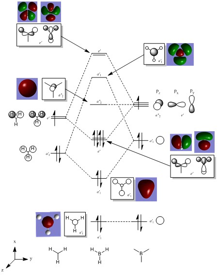
The qualitatively determined molecular orbitals and those calculated computationally show a very high degree of similarity, and thus shows that the qualitative method is a valid approach and gives reliable results. The fact that there are no obvious mismatches between any of the orbitals suggests that the qualitative approach can be a very useful tool as its bypasses the complicated mathematics involved with solving the Schrodinger equation and allows chemists to predict, quite accurately, the shape of molecular orbitals purely based on the combination of pictorally represented atomic orbitals.
Full analysis of NH3
Optimisation
Optimisation of the NH3 molecule was performed using the 6-31G (d,p) basis set. The results are shown below (nosymm keyword was used).The log file can be found here.

| Calc. Type: | Method: | Basis Set: | Energy (Hartree): | Energy (kJmol-1): | RMS Gradient: | Dipole Moment (Debye): | Point Group: |
| FOPT | RB3LYP | 6-31G (d,p) | -56.55776856 | -148490 | 0.000 | 1.85 | C1 |
  Item               Value     Threshold  Converged?
 Maximum Force            0.000024     0.000450     YES
 RMS     Force            0.000012     0.000300     YES
 Maximum Displacement     0.000079     0.001800     YES
 RMS     Displacement     0.000053     0.001200     YES
 Predicted change in Energy=-1.629718D-09
 Optimization completed.
    -- Stationary point found.
                           ----------------------------
                           !   Optimized Parameters   !
                           ! (Angstroms and Degrees)  !
 --------------------------                            --------------------------
 ! Name  Definition              Value          Derivative Info.                !
 --------------------------------------------------------------------------------
 ! R1    R(1,2)                  1.018          -DE/DX =    0.0                 !
 ! R2    R(1,3)                  1.018          -DE/DX =    0.0                 !
 ! R3    R(1,4)                  1.018          -DE/DX =    0.0                 !
 ! A1    A(2,1,3)              105.7413         -DE/DX =    0.0                 !
 ! A2    A(2,1,4)              105.7486         -DE/DX =    0.0                 !
 ! A3    A(3,1,4)              105.7479         -DE/DX =    0.0                 !
 ! D1    D(2,1,4,3)           -111.8631         -DE/DX =    0.0                 !
 --------------------------------------------------------------------------------

 GradGradGradGradGradGradGradGradGradGradGradGradGradGradGradGradGradGrad
Frequency Analysis
A frequency analysis was carried out for the optimised NH3 using the keywords 'int=ultrafine' and 'scf=tight', and submitted to the HPC for the calculation to determine whether or not the energy is at a minimum value. The link to the published files can be found here: DOI:10042/27767 .
| Calc. Type: | Method: | Basis Set: | Energy (Hartree): | Energy (kJmol-1): | RMS Gradient: | Dipole Moment (Debye): | Point Group: |
| FOPT | RB3LYP | 6-31G (d,p) | -56.55776872 | -148490 | 0.000 | 1.85 | C1 |
Low frequencies ---  -10.0166   -0.0005    0.0012    0.0014    9.2679   14.6652
Low frequencies --- 1089.3137 1693.9163 1693.9485

Population Analysis
Population Analysis was carried out by editing the optimised checkpoint file and setting up a calculation with the keyword "pop= full" and submitting it to the HPC. The link to the files is given here: DOI:10042/27768 .
| MO number: | MO number: | ||
| 1 |  |
5 |  |
| 2 |  |
6 |  |
| 3 |  |
7 |  |
| 4 |  |
8 |  |
Natural Bond Orbital Analysis


In order to analyse the natural bond orbitals (NBOs), the log file from the population analysis is required (the checkpoint file was used for MO analysis). The first result we can obtain is the charge distribution, which is shown in Fig. 9, where the colours red and green are used to show regions of negative and positive charge respectively. It is also possible to compute these values as numbers, and the result is shown in Fig. 10: N = -1.1.25 units and H = 0.375 units. Natural bond orbitals can be further analysed by looking at the log text file, from which it is possible to deduce bonding contributions and the energies of the different bonds (and in this case, the lone pair).
Full analysis of NH3BH3
Ammonia-borane (NH3BH3) has been of interest recently due to its potential to store hydrogen as a fuel. It is an example of an acid-base complex, and as the energies of BH3 and NH3 have already been previously computed using the same basis set (BLY3P/6-31G (d, p)),it will be possible to compute the energy of the 'supposed' dative bond as the difference between the energy of the product and the reactants. This energy is also termed an 'association' energy.
Optimisation

NH3BH3 was optimised using the same basis set as for ammonia and borane above. The resulting Gaussian log file can be found here. [[Media:|here]].
| Calc. Type: | Method: | Basis Set: | Energy (Hartree): | Energy (kJmol-1): | RMS Gradient: | Dipole Moment: | Point Group: |
| FOPT | RB3LYP | 6-31G (d,p) | -83.22469048 | -218510 | 0.000 | 5.56 | C1 |
Item               Value     Threshold  Converged?
 Maximum Force            0.000014     0.000015     YES
 RMS     Force            0.000006     0.000010     YES
 Maximum Displacement     0.000054     0.000060     YES
 RMS     Displacement     0.000021     0.000040     YES
 Predicted change in Energy=-1.067687D-09
 Optimization completed.
    -- Stationary point found.
                           ----------------------------
                           !   Optimized Parameters   !
                           ! (Angstroms and Degrees)  !
 --------------------------                            --------------------------
 ! Name  Definition              Value          Derivative Info.                !
 --------------------------------------------------------------------------------
 ! R1    R(1,7)                  1.0185         -DE/DX =    0.0                 !
 ! R2    R(2,7)                  1.0185         -DE/DX =    0.0                 !
 ! R3    R(3,7)                  1.0185         -DE/DX =    0.0                 !
 ! R4    R(4,8)                  1.2098         -DE/DX =    0.0                 !
 ! R5    R(5,8)                  1.2098         -DE/DX =    0.0                 !
 ! R6    R(6,8)                  1.2098         -DE/DX =    0.0                 !
 ! R7    R(7,8)                  1.6677         -DE/DX =    0.0                 !
 ! A1    A(1,7,2)              107.8761         -DE/DX =    0.0                 !
 ! A2    A(1,7,3)              107.8764         -DE/DX =    0.0                 !
 ! A3    A(1,7,8)              111.0236         -DE/DX =    0.0                 !
 ! A4    A(2,7,3)              107.8815         -DE/DX =    0.0                 !
 ! A5    A(2,7,8)              111.0195         -DE/DX =    0.0                 !
 ! A6    A(3,7,8)              111.0198         -DE/DX =    0.0                 !
 ! A7    A(4,8,5)              113.8725         -DE/DX =    0.0                 !
 ! A8    A(4,8,6)              113.8727         -DE/DX =    0.0                 !
 ! A9    A(4,8,7)              104.5966         -DE/DX =    0.0                 !
 ! A10   A(5,8,6)              113.8785         -DE/DX =    0.0                 !
 ! A11   A(5,8,7)              104.5946         -DE/DX =    0.0                 !
 ! A12   A(6,8,7)              104.5984         -DE/DX =    0.0                 !
 ! D1    D(1,7,8,4)           -179.9986         -DE/DX =    0.0                 !
 ! D2    D(1,7,8,5)            -60.0017         -DE/DX =    0.0                 !
 ! D3    D(1,7,8,6)             60.0026         -DE/DX =    0.0                 !
 ! D4    D(2,7,8,4)            -60.0001         -DE/DX =    0.0                 !
 ! D5    D(2,7,8,5)             59.9967         -DE/DX =    0.0                 !
 ! D6    D(2,7,8,6)           -179.9989         -DE/DX =    0.0                 !
 ! D7    D(3,7,8,4)             60.0025         -DE/DX =    0.0                 !
 ! D8    D(3,7,8,5)            179.9993         -DE/DX =    0.0                 !
 ! D9    D(3,7,8,6)            -59.9963         -DE/DX =    0.0                 !
 --------------------------------------------------------------------------------
 GradGradGradGradGradGradGradGradGradGradGradGradGradGradGradGradGradGrad
Frequency Analysis
A frequency analysis was carried out for the optimised NH3BH3 again using the keywords 'int=ultrafine' and 'scf=tight'. The file was submitted to the HPC for the calculation to determine whether or not the energy is a minimum. The link to the published files can be found here:DOI:10042/27781 .
| Calc. Type: | Method: | Basis Set: | Energy (Hartree): | Energy (kJmol-1): | RMS Gradient: | Dipole Moment (Debye): | Point Group: |
| FOPT | RB3LYP | 6-31G (d,p) | -83.22468910 | -218510 | 0.000 | 5.56 | C1 |
Low frequencies ---   -5.1845   -3.8319   -0.0014   -0.0013   -0.0004    3.5935
Low frequencies ---  263.2938  632.9684  638.3944
Association Energy Calculation
To calculate a value for the B-N bond strength, the difference between the energies of the products and reactants can be calculated as shown below:
E(NH3) = -56.55776856 a. u.
E(BH3) = -26.61532361 a. u.
E(NH3BH3) = -83.22468910 a. u.
ΔE = E(NH3BH3) - [E(NH3) + E(BH3)] = -0.05159693 a.u
-0.05159693 a.u. = -135 kJmol-1
The literature value for the dissociation energy is 31 ± 2.6 kcalmol-1, [6] which equates to approximately 130 ± 11 kJmol-1 (note that the bond dissociation energy has the opposite sign to the bond association energy as they are reverse processes). The agreement between this computed value and literature is very good, and shows that this basis set and method combination (DFT 3BLYP and 6-31G (d,p) generates an accurate prediction.
Mini Project: Ionic Liquids- Designer Solvents
In this part of the inorganic computational module, the aim is to investigate a group of compounds known as 'ionic liquids', which are salts that melt at relatively low temperatures (conventionally less than 100 °C but more importantly those that are in the liquid phase at room temperature). It is well known that ionic lattices such as sodium chloride melt at high temperatures, so how can it be possible to obtain room temperature liquid salts? The answer is to use weakly co-ordinating anions- typically a large bulky, modifiable organic cation (e.g. ammonium, imidazolium derivatives) and an inorganic cation (e.g. tetrafluoroborate, halide ions). Given that it is possible to tune the properties of these ionic liquids by choosing the right combination of ions or by modifying the organic groups by alternating the carbon chain lengths, they have been at the forefront of chemical research for the last few decades and have since found applications in electrochemistry,[7] the processing of bio-materials such as cellulose[8] and as solvents[9] to name a few.
In recent years, the phrase 'designer solvents' has been coined to describe, perhaps, the most important application of ionic liquids in the future. Computational chemistry will have an increasingly important rolein predicting the properties of different combinations of weakly co-ordinating anions and determining whether or not they would be suitable alternatives to the volatile organic compounds that are used in most chemical reactions today.
The first part of this exercise will involve the computational analysis of three polyatomic cations and then the second part will involve looking at the effects of having negatively charged ligands (OH- and CN-) as part of the tetraalkylammonium cation framework and any influence that might have on the frontier orbitals generated and the charge distribution.
Optimisation and Frequency Analysis 1
Optimisation calculations were carried out for three polyatomic cations- tetramethylammonium (N(CH3)4+), tetramethylphosphonium (P(CH3)4+) and trimethylsulfonium (S(CH3)3+- using the DFT-BLY3P method and 6-31G (d,p) basis sets and the keywords 'scf=conver=9', 'opt=tight', 'int=ultrafine' and 'nosymm' were added to make the calculation more accurate. Frequency calculations were performed with these same conditions, and all Gaussian input files were uploaded to the HPC. All links can be found below in the relevant sections.
N(CH3)4+
4%2B_geometry_BCHL.png)
Link to the HPC optimisation results:DOI:10042/27803 . Link to the HPC frequency results: DOI:10042/27817 .
| Calc. Type: | Method: | Basis Set: | Energy (Hartree): | RMS Gradient: | Dipole Moment: | Point Group: |
| FOPT | RB3LYP | 6-31G (d,p) | -214.18127322 | 0.000 | 7.63 | C1 |
       Item               Value     Threshold  Converged?
 Maximum Force            0.000000     0.000015     YES
 RMS     Force            0.000000     0.000010     YES
 Maximum Displacement     0.000010     0.000060     YES
 RMS     Displacement     0.000004     0.000040     YES
 Predicted change in Energy=-8.537684D-13
 Optimization completed.
    -- Stationary point found.
| Calc. Type: | Method: | Basis Set: | Energy (Hartree): | RMS Gradient: | Dipole Moment: | Point Group: |
| FREQ | RB3LYP | 6-31G (d,p) | -214.18127322 | 0.000 | 7.63 | C1 |
Low frequencies ---   -5.4466   -2.0911    0.0007    0.0010    0.0011    4.0021
Low frequencies ---  183.7643  288.4013  288.9011
P(CH3)4+
4%2B_geometry_BCHL.png)
Link to the HPC optimisation results:DOI:10042/27804 . Link to the HPC frequency results:DOI:10042/27818
| Calc. Type: | Method: | Basis Set: | Energy (Hartree): | RMS Gradient: | Dipole Moment: | Point Group: |
| FOPT | RB3LYP | 6-31G (d,p) | -500.82701172 | 0.000 | 6.46 | C1 |
         Item               Value     Threshold  Converged?
 Maximum Force            0.000002     0.000015     YES
 RMS     Force            0.000000     0.000010     YES
 Maximum Displacement     0.000034     0.000060     YES
 RMS     Displacement     0.000012     0.000040     YES
 Predicted change in Energy=-5.967853D-12
 Optimization completed.
    -- Stationary point found.
| Calc. Type: | Method: | Basis Set: | Energy (Hartree): | RMS Gradient: | Dipole Moment: | Point Group: |
| FREQ | RB3LYP | 6-31G (d,p) | -500.82701172 | 0.000 | 6.46 | C1 |
Low frequencies ---   -2.4968   -0.0024    0.0022    0.0029    5.2214    7.5761
Low frequencies ---  156.4522  192.0479  192.2848
S(CH3)3+
3%2B_geometry_BCHL.png)
Link to the HPC optimisation results:DOI:10042/27809 . Link to the HPC frequency results: DOI:10042/27819
| Calc. Type: | Method: | Basis Set: | Energy (Hartree): | RMS Gradient: | Dipole Moment: | Point Group: |
| FOPT | RB3LYP | 6-31G (d,p) | -517.68327465 | 0.000 | 5.87 | C1 |
       Item               Value     Threshold  Converged?
 Maximum Force            0.000001     0.000015     YES
 RMS     Force            0.000000     0.000010     YES
 Maximum Displacement     0.000016     0.000060     YES
 RMS     Displacement     0.000005     0.000040     YES
 Predicted change in Energy=-9.671352D-12
 Optimization completed.
    -- Stationary point found.
| Calc. Type: | Method: | Basis Set: | Energy (Hartree): | RMS Gradient: | Dipole Moment: | Point Group: |
| FREQ | RB3LYP | 6-31G (d,p) | -517.68327465 | 0.000 | 5.87 | C1 |
Low frequencies ---   -6.7194   -1.8334   -0.0026   -0.0018    0.0017    7.8396
Low frequencies ---  161.9347  199.5467  200.0678
The optimised geometries are shown above for all three cations. N(CH3)4+ and P(CH3)4+ are shown to have a tetrahedral geometry, with the C-Het-C bond angle being 109.5 ° as expected. S(CH3)3+ only has three substituents, and the optimised C-S-C angle was found to be 102.7 °, which suggests that the structure seems to be based on either a bent or trigonal pyramidal geometry, but perhaps slightly distorted due to the angle being slightly smaller. It is also possible to look at the C-Heteroatom bond lengths to see if there are any noticeable patterns or unexpected results. The C-N bond in N(CH3)4+ was found to be 1.51 Å whereas the C-P bond in P(CH3)4+ had an optimum value of 1.82 Å. N and P are both in Group 15, and it is the expected that going down the group, the bond distance to C will increase as is this case here. This is because the 3p orbitals for P are more diffuse than the N 2p orbitals, and therefore the overlap with the C 2p orbitals will be less efficient, resulting in a weaker, lengthened bond. The optimised S-C bond length was found to be the same as that for P-C (1.82 Å). As sulfur is to the immediate right of P in the periodic table, one would expect that the two bond lengths be quite similar- the orbital sizes do not change much going across the p-block, and the atomic radii for both elements are the same value too,[10] thus the results seem to correlate well with theory.
MO Analysis of N(CH3)4+
The population calculation for N(CH3)4+ was set up using the checkpoint output file from the completed optimisation calculation. The method used was changed from 'optimisation' to 'energy' and the keyword "pop=full" added before the file was uploaded to the HPC. The resultant files can be accessed here: DOI:10042/27820 .
Five visualised molecular orbitals of N(CH3)4+ have been selected for analysis below:


NBO Analysis 1
The natural bond orbitals can be analysed using the .log file generated from the population analysis. The table below summarises the NBO charge distribution of the three cations:
| Cation: | N(CH3)4+ | P(CH3)4+ | S(CH3)3+ |
 |
 |
 |
 |
| Heteroatom Charge/ Debye: | N = -0.295 | P = 1.667 | S = 0.917 |
| Carbon Charge/ Debye: | -0.483 | -1.060 | -0.846 |
| Hydrogen Charge/ Debye: | 0.269 | 0.298 | 0.297 |
Looking at the above results, it is seen that the calculated charges assigned to the heteroatoms reflect their relative electronegativities- nitrogen is the most electronegative of the three elements and has a calculated charge of -0.295 D followed by sulfur with 0.917 D and phosphorus, which has a large positive value (1.667 D). However, whilst it would be expected that carbon is assigned a negative value with respect to phosphorus and sulfur, it is quite unexpected, at a first glance, that it would have a more negative charge than nitrogen.
To explain this, the carbon atom must be considered as being part of a methyl unit. Hydrogen is more electropositive than carbon (H = 2.20, C = 2.55 according to the Pauling Scale) and there are three hydrogens to one carbon atom, and so there will be a net dipole present with the carbon bearing more of the electron density (this is also used to explain why methyl groups are electron-donating). The charge on the hydrogen atoms is of a similar value in all three cations, and so they can be treated as being a constant value for the purpose of this explanation. Carbon is shown to have the greatest charge density when bound to phosphorus- this might be because phosphorus has a high electron density relative to N, C and H and is the least electronegative of the three elements, and so the electrons will orient towards to carbon atom from both P and H atoms. Sulphur also has a relatively high electron density, and as it has a similar electronegativity value to carbon, the electrons will be distributed relatively evenly between the C and S atoms, and the charge on carbon becomes more positive (- 0.846 D). In the case of nitrogen, there is a reasonable difference in electronegativity between nitrogen and carbon, and the nitrogen atom will pull electrons towards itself from all four of the carbon atoms. However, because the nitrogen is withdrawing electrons from four electropositive atoms rather than one atom, the four atoms will contribute equally to the net accumulation of electron density by the nitrogen atom, meaning that each individual carbon atom loses less of their own negative charge and thus the carbons remain more negative than the central nitrogen atom.
Below are results from the .log file showing the relative electron density contributions from carbon and the heteroatom to the C-Het bond:
C-N bond:
     4. (1.98452) BD ( 1) C   1 - N  17
                ( 33.65%)   0.5801* C   1 s( 20.78%)p 3.81( 79.06%)d 0.01(  0.16%)
                                            0.0003  0.4552 -0.0237  0.0026 -0.4057
                                           -0.0172  0.7245  0.0308  0.3157  0.0134
                                           -0.0262 -0.0114  0.0204 -0.0160 -0.0126
                ( 66.35%)   0.8146* N  17 s( 25.00%)p 3.00( 74.97%)d 0.00(  0.03%)
                                            0.0000  0.5000 -0.0007  0.0000  0.3954
                                           -0.0001 -0.7061  0.0001 -0.3077  0.0000
                                           -0.0115 -0.0050  0.0089 -0.0070 -0.0055
C-P bond:
     4. (1.98031) BD ( 1) C   1 - P  17
                ( 59.57%)   0.7718* C   1 s( 25.24%)p 2.96( 74.67%)d 0.00(  0.08%)
                                            0.0002  0.5021  0.0171 -0.0020  0.3542
                                           -0.0065 -0.7055  0.0129  0.3512 -0.0064
                                           -0.0168  0.0084 -0.0167 -0.0125 -0.0073
                ( 40.43%)   0.6358* P  17 s( 25.00%)p 2.97( 74.15%)d 0.03(  0.85%)
                                            0.0000  0.0001  0.5000 -0.0008  0.0000
                                            0.0000 -0.3529  0.0005  0.0000  0.7031
                                           -0.0010  0.0000 -0.3500  0.0005 -0.0535
                                            0.0266 -0.0531 -0.0399 -0.0233
C-S bond:
     4. (1.98631) BD ( 1) C   1 - S  13
                ( 48.67%)   0.6976* C   1 s( 19.71%)p 4.07( 80.16%)d 0.01(  0.14%)
                                            0.0003  0.4437  0.0140 -0.0033  0.7221
                                           -0.0056  0.3845 -0.0030 -0.3636 -0.0098
                                            0.0220 -0.0212 -0.0113  0.0148 -0.0096
                ( 51.33%)   0.7164* S  13 s( 16.95%)p 4.86( 82.42%)d 0.04(  0.63%)
                                            0.0000  0.0001  0.4116 -0.0075  0.0012
                                            0.0000 -0.7166  0.0315  0.0000 -0.3816
                                            0.0168  0.0000  0.4039  0.0260  0.0410
                                           -0.0547 -0.0292  0.0276 -0.0051
These results reinforce the explanation above- the calculations indeed show that carbon contributes more electron density than phosphorus to the C-P bond (approximately 60:40); that carbon and sulfur contribute almost 50:50 to the C-S bond, and that nitrogen contributes more electron density to the C-N bond (34:66).
Tetra-alkylammonium species (NR4+) are often depicted as lewis structures in which the positive charge is placed at the nitrogen atom. The positive charge is a 'formal charge', and can worked out using the equation:
FC = No. Valence electrons-(non bonding valence electrons +Bonding valence electrons/2)
In the case of nitrogen in NR4+: FC = 5- (0 + 8/2) = +1
Given the findings from this computational assignment, this may not be a completely valid assumption as the positive charge is not really located at the nitrogen atom. In Table 22 above, the quantitative charge distribution shows that the methyl hydrogen atoms are the atoms that are assigned the most positive charge. However, if the formal charge equation is applied to hydrogen, the result = 1 -(0 + 2/2)= 0. The reason that the formal charge assignment breaks down and is not valid for this molecule is that the model assumes (for simplicity's sake) that the two atoms involved in forming a bond contribute one electron each (i.e. their contributions are equal), which is rather inaccurate when compared to the data obtained from quantum mechanical calculations. As has been seen, atoms do not necessarily contribute equally to bonds as is the case here, therefore the equation should be applied with caution and seen as a rough approximation of where the charge lies on a molecule.
Optimisation and Frequency Analysis 2
Optimisation calculations were carried out for[N(CH3)3(CH2OH)]+ and[N(CH3)3(CH2CN)]+ using the DFT-BLY3P method and 6-31G (d,p) basis sets and the keywords 'scf=conver=9', 'opt=tight', 'int=ultrafine' and 'nosymm' were used. Frequency calculations were performed under these same conditions, and all Gaussian input files were uploaded to the HPC. All links can be found below in the relevant sections.
[N(CH3)3(CH2OH)]+
Link to the HPC optimisation results:DOI:10042/27859 . Link to the HPC frequency results: DOI:10042/27862 .
| Calc. Type: | Method: | Basis Set: | Energy (Hartree): | RMS Gradient: | Dipole Moment: | Point Group: |
| FOPT | RB3LYP | 6-31G (d,p) | -289.39470674 | 0.000 | 2.18 | C1 |
         Item               Value     Threshold  Converged?
 Maximum Force            0.000003     0.000015     YES
 RMS     Force            0.000000     0.000010     YES
 Maximum Displacement     0.000054     0.000060     YES
 RMS     Displacement     0.000013     0.000040     YES
 Predicted change in Energy=-6.345466D-11
 Optimization completed.
    -- Stationary point found.
| Calc. Type: | Method: | Basis Set: | Energy (Hartree): | RMS Gradient: | Dipole Moment: | Point Group: |
| FREQ | RB3LYP | 6-31G (d,p) | -289.39470674 | 0.000 | 2.18 | C1 |
Low frequencies ---   -8.9661   -7.1888    0.0007    0.0007    0.0010    5.2336
Low frequencies ---  131.0447  214.2459  255.7142
[N(CH3)3(CH2CN)]+
Link to the HPC optimisation results:DOI:10042/27825 . Link to the HPC frequency results: DOI:10042/27827 .
| Calc. Type: | Method: | Basis Set: | Energy (Hartree): | RMS Gradient: | Dipole Moment: | Point Group: |
| FOPT | RB3LYP | 6-31G (d,p) | -306.39376383 | 0.000 | 5.76 | C1 |
        Item               Value     Threshold  Converged?
 Maximum Force            0.000000     0.000015     YES
 RMS     Force            0.000000     0.000010     YES
 Maximum Displacement     0.000004     0.000060     YES
 RMS     Displacement     0.000001     0.000040     YES
 Predicted change in Energy=-7.474396D-13
 Optimization completed.
    -- Stationary point found.
| Calc. Type: | Method: | Basis Set: | Energy (Hartree): | RMS Gradient: | Dipole Moment: | Point Group: |
| FREQ | RB3LYP | 6-31G (d,p) | -306.39376383 | 0.000 | 5.76 | C1 |
Low frequencies ---   -2.6414   -0.0009   -0.0008   -0.0006    7.1436    9.6692
Low frequencies ---   91.7729  154.0265  210.9283
NBO Analysis 2
The population calculations were carried out using the same method described in previous section of the mini project. Links to population analysis are provided here-
[N(CH3)3(CH2OH)]+: DOI:10042/27924 and [N(CH3)3(CH2CN)]+: DOI:10042/27830 . The table below shows the calculated charge distributions of the two cations:
| Cation: | [N(CH3)3(CH2OH)]+ | [N(CH3)3(CH2CN)]+ |
 |
 |
 |
| Quantitative Charge Distribution: |  |
 |
| Central N Charge/ Debye: | -0.322 | -0.289 |
| Methyl Carbons Charge Range/ Debye: | -0.491 to -0.494 | -0.485 to -0.489 |
| Methyl Hydrogens Charge Range/ Debye: | 0.262 to 0.282 | 0.269 to 0.282 |
| CH2 Charges/ Debye: | C = 0.088, H = 0.237, 0.249 | C = -0.350, H = 0.309 |
| Ligand Charges/ Debye: | O = -0.725, H = 0.521 | C= 0.209, N = -0.186 |
The two chosen ligands alter the charge distribution of the ammonium ion in slightly different ways. OH- is an example of an electron-donating group, and the oxygen atom is calculated to have the largest negative charge (-0.725 D). The carbon adjacent to the oxygen atom carries a positive charge (0.088 D), which is due to being bonded to two electronegative atoms, but there are not many other changes in the charge distribution. On the other hand, CN- is an electron-withdrawing functional group. The charge distribution changes more drastically in this case as the nitrogen in the nitrile group has a negative charge of -0.186 D and accepts electron density from the carbon it is bonded to, thus making it become positively charged (0.209 D). Because this carbon is now electron deficient with respect to the methylene carbon, and the continual electron withdrawing effect of the nitrogen atom, electrons move from the methylene carbon to the nitrile group. Consequently, this carbon becomes slightly more positively charged than in the case with N(CH3)4+ (-0.35 D vs. -0.49 D in N(CH3)4+).
HOMO/LUMO Analysis:
| Cation: | N(CH3)4+ | [N(CH3)3(CH2OH)]+ | [N(CH3)3(CH2CN)]+ |
| LUMO: |  |
 |
 |
| LUMO Energy/ a.u. : | -0.13301 | -0.12459 | -0.18183 |
| HOMO: |  |
 |
 |
| HOMO Energy/ a.u. : | -0.57934 | -0.48762 | -0.50048 |
| HOMO-LUMO gap/ a.u. : | 0.44633 | 0.36303 | 0.31865 |
| HOMO-LUMO gap/ kJmol-1 : | 1172 | 953 | 837 |
The table above shows the changes in the orbital shape, energies and size of the HOMO-LUMO gap upon addition of a negatively charged ligand. In the case with [N(CH3)3(CH2OH)]+, the LUMO energy increases and becomes more antibonding. Looking at the visualised LUMO, the introduction of the OH group enables a moderately strong through-space bonding interaction but the red-phase becomes enveloped by the greater delocalised green-phase and this causes strong antibonding interactions to be present. The HOMO is also raised in energy as the atomic orbitals which are in the same phase are now more spread out, leading to a decrease in the strength and number of bonding interactions. However, the HOMO-LUMO gap decreases from N(CH3)4+, which means that it would potentially be more reactive as the energy needed to excite an electron to the LUMO decreases.
For [N(CH3)3(CH2CN)]+, the LUMO decreases in energy compared to the tetra-methylammonium cation. From the visualised LUMO, it can be seen that the red phase orbitals are closer together and this will increase the bonding interactions present in the MO. The HOMO increases in energy compared to N(CH3)4+ and this, as for the previous molecule, is due to the decreased number of bonding interactions and the increase in strong antibonding interactions. The HOMO-LUMO gap is also decreased from the tetra-methylammonium cation.
Research has shown that it is the cation design that often determines the HOMO-LUMO gap of ionic liquids,[11] thus it is important to consider how large the energy gap is. For their application as solvents, a large HOMO-LUMO gap would lead to increased stability and poorer reactivity, whereas a smaller HOMO-LUMO gap could aid increase the efficiency of processes such as solvent-assisted relaxation. The two examples above show that both electron-withdrawing and electron-donating groups will have a tendency to decrease the HOMO-LUMO gap, although the individual frontier orbitals energy levels may be raised or lowered depending on how the molecular orbitals are affected by incorporation of the specific functional group.
References
- ↑ B. Réffy, M. Kolonits and M. Hargittai, J. Mol. Struct., 1998, 445, 139
- ↑ J. C. Slater, J. Chem. Phys., 1964, 41, 3199
- ↑ D. G. de Oteyza, P. Gorman, Y. Chen, S. Wickenburg, A. Riss, D. Mowbray, G. Etkin, Z. Pedramrazi, H. Tsai, A. Rubio, M. Crommie and F. R. Fisher, Science, 2013, 340, 1434
- ↑ K. Kawaguchi, J. E. Butler, C. Yamada, S. Bauer, T. Minowa, H. Kanamori and E Hirota, J. Chem. Phys., 1987, 87, 2438
- ↑ K. Nakamoto, Infrared spectra of inorganic and coordination compounds, Wiley, 1963, 128
- ↑ R. Potter, D. Camaioni, M. Vasiliu and D. Dixon, Inorg. Chem., 2010, 49, 10512
- ↑ H. Liu, Y. Liu, and J. Li, Phys. Chem. Chem. Phys., 2010, 12, 1685
- ↑ S. Zhu, Y. Wu, Q. Chen, Z. Yu, C. Wang, S. Jin, Y. Ding, and G. Wu, Green Chem., 2006, 8, 325
- ↑ J. P. Hallett and T. Welton, Chem. Rev., 2011, 111, 3508
- ↑ J. C. Slater, J. Chem. Phys., 1964, 41, 3199
- ↑ K. Kanai, T. Nishi, T. Iwahashi, Y. Ouchi, K. Seki, Y. Harada and S. Shin,Journal of Electron Spectroscopy and Related Phenomena, 2009, 174, 110