
Rep:Mod:hjw13liquids
Introduction to Molecular Dynamics Simulation
Harmonic Oscillator
Classically, the energy of a simple harmonic oscillator is given by the sum of kinetic energy (given by ) and potential energy (given by where k is the spring constant and x is the displacement from the equilibrium point). By substituting the values of positions and velocity given by the algorithm, the total energy of the system was calculated. Assuming no damping forces, the energy should remain constant.
The absolute difference in position between the analytical and Velocity-Verlet algorithm's solutions were taken in order to reveal the accuracy of the algorithm. It can be seen that oscillations in the error occur with time with error at the maxima increasing greatly with time. By plotting the error only at the maxima, it is shown that the accuracy of the algorithm diminishes with a linear relationship between error at the maxima and time of calculation. This can be rationalised by the fact that every calculation has a small error within it and these errors accumulate over time.
-
 Error over time
 -
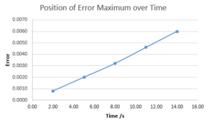 Error maxima over time


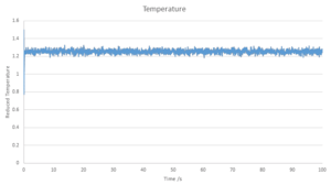
Using a timestep of 0.2s gave an error of 1% for the Velocity-Verlet algorithm from the analytical. Monitoring the total energy of the system is done as, for the simple harmonic oscillator system, the total energy should remain constant as the energy is only exchanged between kinetic and potential energies. This fact can be used to quickly see if an approximation is valid, for example, is the system progressively loses energy, the approximation is invalid.
-
 Variation of Energy over time with V.V algorithm

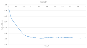
This graph shows that, while the energy does change, it changes periodically around a single value, so this aproximation can be seen as valid in this respect
Lennard-Jones
At zero potential energy, the equilibrium separation, , this is also true also if approaches infinity.
The interatomic force is given by the derivative of potential energy with respect to position:
If done for :
Separation occurs with the interatomic force equals zero which occurs at the minimum of the Leonard-Jones Potential.
is given by:
The well depth is given by substituting into the Leonard-Jones Potential, which gives an answer of . Therefore, to fully dissociate 2 atoms, an energy of must be supplied.
The integrals are solved by substituting the relevant limits into the indefinite integral of the Leonard-Jones Potential:
Periodic Boundary Conditions
The standard molar volume of water is 18mL/mol , multiplication by Avogadro's number gives the number of atoms per milliliter, giving the answer of
Diving 10,000 by this number gives the volume of 10,000 water molecules, the answer to this being
These numbers displays why realistic volumes are not simulated in our calculations, even a single millilitre of liquid would give a huge number of operations that must be done in the calculation, beyond the ability of the computational power and time available to us, therefore, a small number of atoms is chosen for the calculations and the Periodic Boundary Conditions applied.
A particle at (0.5, 0.5, 0.5) in a (1, 1, 1) box moving on vector (0.7, 0.6, 0.2), under the periodic boundary condition, would end up at point (0.2, 0.1, 0.7).
Truncation
In real units, the Leonard-Jones is 1.088nm, the well-depth is -0.998 kJ/mol and the temperature is 180K
Equilibration
Creating the Simulation Box
Randomly assigning starting positions can lead to issues because, if atoms are created too close together, the there would be a very high energy at the start of the simulation which could lead to unrealistic results, the same effect would apply if the randomisation outputted a large space with no molecules in it.
A number density of 0.8 gives lattice volume of 1/0.8 = 1.25, since it is cubic, cube root of volume gives lattice side length, cube root(1.25)=1.07722.
Using a number density of 1.2, and given that a FCC lattice has 4 lattice points and the volume is the number of lattice points divided by the number density of points. Taking the cube root of this volume gives a lattice parameter of 1.49.
Due to the FCC having 4 lattice points, the line "create atoms 1 box" line would gives 4000 atoms if a FCC lattice were used.
Setting Properties of the Atoms
mass 1 1.0
This line sets the mass of atom type 1 (all atoms the same type in this simulation) to 1.0
pair_style lj/cut 3.0
Sets how pairwise interactions are handled by LAMMPS. lj/cut gives the style, 3.0 gives the argument of the style. lj/cut gives a style of cutoff Lennard-Jones potential with no Coulomb and 3.0 is the cutoff point in distance units.
pair_coeff * * 1.0 1.0
This line gives the pairwise force field coefficients between particular atom types. If more than one atom type was used, there would be the numbers of the atoms in place of the asterisks. Instead, the asterisks defines all atoms between 1 and N where N is the total number of atom types. The 1.0 terms give the arguments for each atomic pair type.
As the initial conditions are x(0) and v(0) are specified, the Velocity-Verlet Algorithm can be used.
The lines
timestep 0.001
run 100000
would give the same results in this particular simulation, however this calculation would not give any information on the parameters of the simulation and would not be applicable to any simulations with variable timesteps so the other lines are preserved.
Checking Equilibration
-
 Energy
 -
 Temperature
 -
 Pressure
 -
 Zoom
Zoom


Plots of the reduced energy, temperature and pressure as a function of time are seen in the above graphs, with a time step of 0.001 used, it cna be seen for all cases that the calculations converged around mean values, with variation around the values. By inspecting the zoomed in graph of energy, it can be seen that with a time step of 0.001, the system reaches equilibrium within 0.4.
-
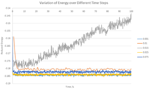 Variation of energy with time step

It can be seen from the combined graph of different time steps that using a time step of 0.015 is unfeasible as system clearly does not reach an equilibrium value within the simulation time. The time steps of 0.001 and 0.0025 converged at values very close to each other whereas 0.01 and 0.0075 gave slightly different equilibrium values meaning that they may give erroneous results if used for further calculations. For these reasons, a time step of 0.001 was used and it gives an accurate calculation while taking less calculation time than 0.0025.
Running Simulations Under Specific Conditions
Temperature and Pressure Control
Thermostats and Barostats
As gamma is not a constant in the summation, it can be pulled out allowing it to be determined in terms of t and tau.
Nevery, Nrepeat and Nfreq
100 in a script is a quantity called Nevery, this directs the calculation to use the given input values every 100 time steps.
1000 in the script is Nrepeat, this gives the number of times to use the input values for the mean
100,000 in the script is Nfreq giving the command to calculate the average after 100,000 time steps and is found by getting the product of Nevery and Nrepeat
Equations of State
The ideal gas law is:
Rearranging this in terms of gives:
As in the reduced units system, all constants are set to 1, the Ideal Gas Law can give a prediciton for the density of the system.

It can be clearly seen that the ideal gas law predicts higher densities than those given by the Velocity Verlet Algorithm. This is easily rationalised when considering the assumptions of the Ideal Gas Law, namely that the particles involved can be treated as point-like and do not interact with each other. Other than the obvious fact that this have issues when applied to a liquid system, this model also doesn't give any repulsive forces between particles upon applied pressure so atoms can approach each other without a lower limit. Molecular Dynamics, however, models the interactions with interatomic potentials such as the Leonard-Jones which is the potential used here. |As atoms approach each other less than the equilibrium distance, an overall repulsive force begins to take effect, increasing proportionally to 1/r^{12}, ensuring that the particles do not reach distances below /sigma. Density could be more accurately modeled for this system with the Van Der Waals Equation, a model that takes into account atomic volumes and interatomic interactions.
The difference between the two methods reduces at higher temperature due to the Ideal Gas Law's prediction reducing at a faster rate than the Velocity-Verlet Algorithm. It is also observed that a larger pressure gives a higher density, which is expected for the vast majority of systems.
Calculating Heat Capacities Using Statistical Physics
The input code for the following simulations is given below:
### DEFINE SIMULATION BOX GEOMETRY ###
variable den equal 0.8
lattice sc ${den} ### defines den as a variable
region box block 0 15 0 15 0 15
create_box 1 box
create_atoms 1 box

### DEFINE PHYSICAL PROPERTIES OF ATOMS ###
mass 1 1.0
pair_style lj/cut/opt 3.0
pair_coeff 1 1 1.0 1.0
neighbor 2.0 bin

### SPECIFY THE REQUIRED THERMODYNAMIC STATE ###
variable T equal 2.0 ### temperature  and time step varied, pressure not used anymore
variable timestep equal 0.01

### ASSIGN ATOMIC VELOCITIES ###
velocity all create ${T} 12345 dist gaussian rot yes mom yes

### SPECIFY ENSEMBLE ###
timestep ${timestep}
fix nve all nve

### THERMODYNAMIC OUTPUT CONTROL ###
thermo_style custom time etotal temp press
thermo 10

### RECORD TRAJECTORY ###
dump traj all custom 1000 output-1 id x y z

### SPECIFY TIMESTEP ###

### RUN SIMULATION TO MELT CRYSTAL ###
run 10000
unfix nve
reset_timestep 0

### BRING SYSTEM TO REQUIRED STATE ###
variable tdamp equal ${timestep}*100
fix nvt all nvt temp ${T} ${T} ${tdamp}
run 10000
reset_timestep 0

### MEASURE SYSTEM STATE ###
thermo_style custom step etotal temp density
variable erg equal etotal
variable erg2 equal etotal*etotal
variable temp equal temp
variable temp2 equal temp*temp
fix aves all ave/time 100 1000 100000 v_temp v_erg v_erg2
unfix nvt
fix nve all nve ###added as in script
run 100000

variable avetemp equal f_aves[1]
variable heatcapacity equal (atoms*atoms*(f_aves[3]-f_aves[2]*f_aves[2]))/(${avetemp}*${avetemp}*vol) ### gives heat capacity over volume

print "Averages"
print "--------"
print "Temperature: ${avetemp}"
print "Heat Capacity over Volume : ${heatcapacity}"

Heat Capacity is an extensive property of a system which is defined as the energy required per unit increase of temperature. Heat capacities tend to increase or remain constant with respect to temperature due to the fact that, at higher energies, the energy difference between the states decreases, lowering the energy required for excitation , increasing the change in temperature for a given energy input. There comes a point at higher temperature that the energy in the atoms allows interchange between states without need for extra energy input, this decreases the systems ability to absorb supplied energy, decreasing heat capacity. The fact that Heat capacity is an extensive property of a system, it is expected that a higher density gives a larger heat capacity per unit volume, as there are more atoms per unit volume to absorb energy.
Thermal expansion of phases tends to occur with increasing temperature. Owing to the fact that the heat capacity has been divided by volume, the reduction in heat capacity over volume, with respect to temperature, was exaggerated. Expansions occur at larger temperatures because atoms have larger translational and vibrational motion.
Structural properties and the radial distribution function
To simulate each of the phases for the simulation, the following densities and temperatures were used:
Solid: D = 1.1, T = 1.0
Liquid: D = 0.8, T = 1.2
Gas: D = 0.4, T = 1.5
These gave the results for g(r) and the running integral of g(r)


All phases have zero g(r) below a radius of one, this is as expected as a radius of 1 corresponds to the radius of one atom. Therefore, anything appearing below r=1 would indicate an overlap of atoms which obviously cannot occur. After this point, the g(r) for all phases increases to a maximum shortly after, before dropping and oscillating towards a value of 1, which is the point that the RDF of the bulk has been normalised to. The solid phase has the highest maximum of the three and takes the longest to normalise, in fact the oscillations are still observed within the time frame of the simulation. The vapour phase has the shortest period of oscillation and the smallest maximum of g(r), with the liquid phase being intermediate between the two. The solid
The oscillatory nature of the g(r) for the liquid and solid phases indicates that they form shells and that the atoms tend to take constant positions relative to each other. As this order is not observed in the vapour phase, it can be assumed that these shells do not form. The larger oscillations observed for the solid phase over the liquid are observed due to the fact that the atoms are packed in a periodic, stationary structure whereas the atoms in the liquid phase are in constant motion and so form more dynamic shells.
The g(r) for the solid show well defined peaks and valleys indicating well defined positions with only small variation around each point, and little density between them This is expected for a strongly held periodic lattice. the first, largest peak at r*=1.025 corresponds to the closest neighbour in the FCC lattice, the distance between the lattice point and the atom in the face of the cube. The following peaks at 1.475 and 1.825 correspond to the next closest interaction which are the distances between the lattice points between two layers in the lattice, and between the lattice point and the atom in the centre of the above face respectively.
The running integral of g(r) was also calculated. This integral corresponds to the number of atoms represented by the g(r). As could be expected, the solid has the largest integral due to it having the highest density of the three phases, with liquid following after.
By examining the integral for the solid curve for each of the three first peaks, the number of atoms represented at each distance can be calculated and therefore, the number of nearest neighbours can be calculated. The number of atoms represented by the first peak was found to be 12, giving the number of nearest neighbours. The second and third peaks were found to represent 6.5 and 23.8 atoms respectively.
Diffusion Coefficient
Mean Squared Displacement


The above graphs display the change mean squared displacement over time for an 8,000 atom system. It is expected, and observed, that, due to the decrease in order when going from solid to vapour, the mean square displacement of a vapour is higher than for a solid or liquid. This is due to the atoms in the vapour phase having large translational velocities and near negligible interatomic interactions. Liquid and solid have fairly similar ranges for mean square displacement with liquids being slightly higher due to the lack of long range order in a liquid system.


These graphs give the same quantities as before, but with a 1,000,000 atom system instead of 8,000 atoms. It can be seen that the graphs are very similar for the gas and liquid phases but the solid, instead of steadily increasing, increases greatly at the start before converging to a value of 0.02. This could be explained by considering the meaning of the mean squared displacement. The MSD is obtained by summing the squares of the displacement of each atom, the purpose of the squaring is to ensure that the displacements in different directions do not cancel each other out. As the MSD is added to the previous time step each time, the final MSD is proportional to the total distance covered by the average particle, giving its proportionality to the Diffusion coefficient. Considering this, plotting MSD over the time step should give a straight line, as is seen for both liquid and gas. However, in the solid system, there should not be any displacement as the particles are assigned to a periodic lattice, with only some fluctuations. The fluctuations give the initial rise in MSD for the system before reaching an average value. Therefore, the 8,000 atom system is sufficient to describe the liquid and vapour phases but not the solid.
The values obtained for the Diffusion coefficient for both systems are shown below.
| Phase | D (8K) | D (Million) |
|---|---|---|
| Solid | ||
| Liquid | ||
| Vapour |
Velocity Autocorrelation Function
Using the equation of position for a simple harmonic oscillator, taking a derivative with respect to time gives the velocity as a function of time
Substituting this into the integral for the velocity autocorrelation function gives:
Using the addition formula of sine for the sine function and splitting into two separate fractions to simplify the integral gives:
As the integral of an odd function between two limits that are equidistant from zero, is equal to zero, this simplifies further to:


The above graphs show the Velocity Autocorrelation function applied to vapour, liquid and solid phases. A single minimum is observed for the liquid phase, near the start of the calculation. For the solid system, after a large minimum at the start, there is a continuing oscillation which corresponds to that found for a simple harmonic oscillator. Both the liquid and solid systems converge to zero, however the liquid system has no observable oscillation past the beginning minimum, it can be seen that the atoms in a liquid system do not influence their neighbours as much as in the solid system. This is due to the fact that the positions of atoms are not fixed in a liquid and the interatomic forces are weaker.
The large difference between the Leonard-Jones and VACF Harmonic Oscillator systems is due to differing behaviour at large displacements. The Leonard-Jones gives a potential energy the approaches zero at large separation due to weakening of interatomic forces, whereas the VACF Harmonic Oscillator predicts an increase of force at large displacement, keeping the atoms close together and their velocities correlated.


The integral of the VACF shown above, being proportional to the diffusion coefficient, displays that the vapour phase has a much larger Diffusion coefficient than either the liquid or solid phases as is expected. Comparing the results ofr diffusion coefficient found for the 8000 and 1,000,000 systems shows a lot of discrepancy, this could be due to different values for each method used to give the vapour and solid systems.
| Phase | D (8K) | D (Million) |
|---|---|---|
| Solid | ||
| Liquid | ||
| Vapour |
There are two possible sources of error in the calculation, the use of the trapezium rule to approximate the integral, and the calculation method itself. The use of the trapezium rule as an approxiamtion can be justified to give relatively little error as the number of data points used is large enough to give a very small linewidth. However, by the curvature of the lines, it canbe seen the the estimate of the Diffusion coefficient given by the trapezium rule would be an underestimate.The error in the calculation itself could only be examined by comparison with other calculation methods and theory so is beyond the scope of this experiment.