
Rep:Mod:gf609mod3
Physical Computational Chemistry
Introduction
Module 3 will be used to study the transition states in larger molecules. Methods based on molecular orbitals will be applied to solve the Schrödinger equation numerically and locate the transition state structures of these larger molecules based on the shape of a PES. It is also possible to calculate reaction paths and barrier heights. The computational chemistry used will investigate the Cope rearrangement and Diels Alder cycloaddition reactions.
In previous modules the molecular mechanics and force field methods used did not describe bond breaking and making or the changes in electron distribution and bonding type. These will therefore not be used in module 3 and instead the molecular orbital approach will be applied.
The Cope Rearrangement
This section will investigate the Cope Rearrangement of 1,5-cyclohexadiene. The preferred reaction mechanism will be found by locating the low energy minima and transition state structures.
The Cope rearrangement is an example of a pericyclic reaction in which electrons move simultaneously in a concerted manner breaking and making bonds. A key feature of pericyclic reactions is the cyclic transition state. The Cope Rearrangement that will be focused on is the [3,3]-sigmatropic shift rearrangement which occurs via a chair or boat transition structure. It has been found that the chair transition state is lower in energy than the boat transition state by 5-6kcal/mol [1].

Computational calculations will be carried out to find the lowest energy conformation of 1,5-cyclohexadiene.
Optimisation Analysis
Initially it is important to first find the lowest energy structures of 1,5-hexadiene, since these are the most stable structures found at a given temperature. The lowest energy structures of butane can be used as a reference for this, and the graph below shows the relative energy of butane as the molecule rotates around the central carbon-carbon bond. The conformations with the lowest energies (ie minima on the graph) will be the conformations that will be investigated further.

The graph above shows that the antiperiplanar and gauche arrangement of the methyl groups in butane are the lowest energy conformations, with dihedral angles of 180˚ and 60˚ respectively. The antiperiplanar conformation is slightly lower than that of the gauche. This is explained by the better overlap of orbitals associated with the antiperiplanar due to the favourable alignment of the orbitals. From this it can be assumed that these two conformations are also the lowest energy conformations for 1,5-hexadiene, and these will therefore be investigated further.
GaussView was used to create four anti conformations and six gauche conformations of 1,5-hexadiene, by altering the antiperiplanar and gauche linkage of the four central carbon atoms. The structure was ‘cleaned up’ and then optimised in Gaussian. The method used for the optimisation was the Hartree Fock and the basis set was set to 3-21G. The %mem was changed to 250MB. Once the optimisation job was finished the checkpoint file was opened and the summary of the optimisation was viewed. This showed the calculated energies of the various structures. The point group of each structure was found by selecting symmetrize in the edit menu. The table below shows the different conformations and their relative energies (1 Ha = 627.5 kcal mol-1). The summaries can also be found by clicking on the link.
Energy and Point Group for 1,5-Hexadiene Conformations| Conformation and Jmol | Structure | Total Energy (HA) | Total Energy (kJ/mol) | Point group |
|---|---|---|---|---|
 |
-231.69260 | 0.04 | C2 | |
 |
-231.69253 | 0.08 | Ci | |
 |
-231.68907 | 2.25 | C2h | |
 |
-231.69097 | 1.06 | C1 | |
 |
-231.68772 | 3.10 | C2 | |
 |
-231.69167 | 0.62 | C2 | |
 |
-231.69266 | 0.00 | C1 | |
 |
-231.69153 | 0.71 | C2 | |
 |
-231.68962 | 1.91 | C1 | |
 |
-231.68916 | 2.20 | C1 |
It can be seen that the Gauche 3 conformation has the lowest energy, and the Anti 1 and Anti 2 structures have the next lowest energies. The data collected draws a different conclusion to that of the graph of the butane conformations which suggests that the antiperiplanar structures have the lowest energies. Since the results from the calculation were unexpected, these three conformations’ geometries were optimised further by using the DFT B3LYP method and 6-31G(d) basis set. This is a more advanced level of theory and therefore the results from this can be thought of as more accurate than the previous geometry optimisation calculations. The calculations were sent to SCAN. The relative energies are shown in the table below:
(DFT-B3LYP/6-31G(d))Energy and Point Group for the three 1,5-Hexadiene Conformations with the lowest energies| Conformation and Jmol | Structure | Total Energy (HA) | Total Energy (kJ/mol) | Point group |
|---|---|---|---|---|
 |
-234.61180[2] | 0.00 | C2 | |
 |
-234.61170[3] | 0.06 | Ci | |
 |
-234.61133[4] | 0.29 | C1 |
The results are interesting since the conformation with the lowest energy is that of Anti 1. This is different to the initial optimisation and demonstrates the importance of method and basis sets to give an accurate outcome. Anti 2 is the second lowest energy conformation and Gauche 3 is now the highest energy conformation of the three. The results are similar to the theoretical predictions made from the butane conformation graph. It is also noticeable that the more sophisticated method of optimisation has calculated energies that are lower than the HF/3-21G optimisation by approximately 3 Ha. The two optimisation calculations take into consideration different parameters. The results show that even for a simple molecule such as 1,5-hexadiene, there is still a difference in the calculated predictions and this difference would become more evident as the larger and more complex molecules were analysed.
Frequency Analysis
The final energies calculated in optimising the geometries represent the energy of 1,5-hexadiene on the bare potential energy surface. Frequency calculations were carried out to characterise the critical point. From the B3LYP/6-31G(d) optimised structure, the frequency was calculated using the same level of theory in SCAN. The completed job was then opened in a log file and the vibrations of the different conformations were animated. There were no imaginary frequencies (negative values) when looking at the table of stretching frequencies which suggests that energy global minima was obtained. The table below shows the key vibrational modes of the three conformations. The IR spectrum and animated vibrations can also be viewed by clicking on the appropriate link:
| Conformation | IR Spectrum | Vibrational Mode | Stretching Frequency (cm-1) | Intensity |
|---|---|---|---|---|
| Anti 1[5] | IR Spectrum |  |
1731.42 | 4.69 |
| Anti 1[6] | IR Spectrum |  |
1734.35 | 13.54 |
| Anti 2[7] | IR Spectrum |  |
1730.95 | 0.00 |
| Anti 2[8] | IR Spectrum |  |
1734.25 | 18.14 |
| Gauche 3[9] | IR Spectrum |  |
1731.86 | 6.89 |
| Gauche 3[10] | IR Spectrum |  |
1732.97 | 6.13 |
All conformations had the vibrational modes associated with a linear hydrocarbon; the C-H rock, stretch and bend and C-C vibrational modes. The vibrational modes that have been focused on in the table above are of the C=C. Literature states that the stretching frequency values should be between 1680-1620 cm-1[11], which is slightly different to those calculated. The asymmetric and symmetric vibrational modes of the two anti conformations are shown, with the asymmetric at a higher wavenumber. The gauche conformation shows the asymmetric and symmetric vibrational modes at similar wavenumbers as the anti conformations and has the asymmetric at a higher wavenumber. The difference between the gauche and anti is the degree of stretching of the two C=C bonds. This is best seen in the gauche animations where one C=C bond stretches more than the other. An explanation for this may be the gauche conformation symmetry.
Thermochemical Analysis
The output file from the frequency calculations was looked at, in particular the thermochemistry section relating to the different conformers. The thermochemical data for the anti 1, anti 2 and gauche 3 is shown below the explanation[12] of the values:
(i) The sum of electronic and zero point energies: E=Eelec +ZPE This is the potential energy at 0K including the zero point vibrational energy.
(ii) The sum of electronic and thermal energies: E=E + Evib +Erot + Etrans This is the energy at 298.15K and 1atm of pressure.
(iii) The sum of electronic and thermal enthalpies: This contains an additional correction for RT (H= E +RT) which is important for dissociation reactions
(iv) The sum of electronic and thermal free energies: This contains an entropy contribution to the free energy G = H – TS.
Anti 1 Thermochemistry Data (Ha) at 298.15k

Sum of electronic and zero-point Energies=           -234.469286
 Sum of electronic and thermal Energies=              -234.461965
 Sum of electronic and thermal Enthalpies=            -234.461021
 Sum of electronic and thermal Free Energies=         -234.500162
Anti 2 Thermochemistry Data (Ha) at 298.15k

Sum of electronic and zero-point Energies=           -234.469212
 Sum of electronic and thermal Energies=              -234.461856
 Sum of electronic and thermal Enthalpies=            -234.460912
 Sum of electronic and thermal Free Energies=         -234.500821
Gauche 3 Thermochemistry Data (Ha) at 298.15K

Sum of electronic and zero-point Energies=           -234.468693
 Sum of electronic and thermal Energies=              -234.461464
 Sum of electronic and thermal Enthalpies=            -234.460520
 Sum of electronic and thermal Free Energies=         -234.500105
The frequency was also calculated at a different temperature (0K) by using Freq=ReadIsotopes in the addition keywords and by changing the temperature value in the input file to 0.00001K. The calculation was sent to SCAN [13][14][15]. The thermochemistry data is shown below:
Anti 1 Thermochemistry Data (Ha) at 0k

Sum of electronic and zero-point Energies=           -234.468848
 Sum of electronic and thermal Energies=              -234.468848
 Sum of electronic and thermal Enthalpies=            -234.468848
 Sum of electronic and thermal Free Energies=         -234.468848
Anti 2 Thermochemistry Data (Ha) at 0k

Sum of electronic and zero-point Energies=           -234.468775
 Sum of electronic and thermal Energies=              -234.468775
 Sum of electronic and thermal Enthalpies=            -234.468775
 Sum of electronic and thermal Free Energies=         -234.468775
Gauche 3 Thermochemistry Data (Ha) at 0k

 Sum of electronic and zero-point Energies=           -234.468256
 Sum of electronic and thermal Energies=              -234.468256
 Sum of electronic and thermal Enthalpies=            -234.468256
 Sum of electronic and thermal Free Energies=         -234.468256
When the calculations were carried out at 0K all the four values were identical. This is as expected since there is no heat energy to contribute to the values, therefore it is only the zero point energy that is seen.
At 298.15K the values change since thermal energy must be accounted for. Therefore as the temperature increases any value with thermal contribution will increase. Thermal free values will decrease as the temperature increases and this can be explained by G=H-TS, ie as the temperature increases the free energy decreases.
With more time it would be interesting to vary the pressure to see how it would affect the values.
Optimising the Chair and Boat Transition Structures
The boat and chair transition states will now be investigated to see which one the reaction occurs by. Optimisations to transition states are more complex than optimisations to a minimum, since it is necessary for the calculation to know where the reaction co-ordinate is. The first way in which a transition state structure can be optimised is by computing the force constant matrix (or Hessian) in the initial step of optimisation and then updating it throughout the optimisation. This is an easy way to optimise the transition state if the guess transition state is close enough to the exact structure. Therefore this method can be used for a simple chair transition state optimisation, giving reliable results.
An alternative method to generate a transition structure is to first freeze the reaction co-ordinate whilst the rest of the molecule is minimised. After, the reaction co-ordinate can be unfrozen and the structure optimised to a transition state structure. This method can save time since it is not always necessary to compute the whole force constant matrix.
Initially an allyl fragment was drawn in GaussView and its geometry optimised using the Hartree Fock method and 3-21G basis set. A new window was opened and the optimised structure was copied twice into it. The two fragements were then arranged to a ‘guess’ chair transition state structure with the distance between the terminal carbons set to 2.20A.
The guess transition state structure underwent a Opt+Freq calculation where it was optimised to a TS (Berny). The force constants were calculated once and the additional keywords ‘Opt=NoEigen’ were added. This stops the calculation crashing if more than one imaginary vibration is found through optimisation. The calculation was sent to SCAN. The vibrations of the completed job were viewed. An imaginary vibration at -818cm-1 is animated below and corresponds to the cope rearrangement. The bond distance between the terminal carbons is 2.02A.

The transition structure was then optimised by the alternative method – the freeze co-ordinate method. The guess structure was copied into a new window and the Redundant Coord Editor was opened. The ‘Create a New Coordinate’ button was selected and the two terminal carbons (which in the rearrangement form/break) were highlighted. ‘Bond’ and ‘Freeze Coordinate’ were selected in the Redundant Coord Editor and the bond distance was set to 2.2A. The button was selected again and the same process was carried out for the other two terminal carbons. A optimisation to a minimum calculation was then carried out under the same method and basis set as before.
The chk file of the finished job showed a structure similar to the structure optimised previously, however the bond distances were set to 2.2A. The Redundant Coord Editor was opened up again and the bonds that were previously frozen were unfrozen and ‘Derivative’ was selected. An Opt+Freq calculation was carried out where thw structure was optimised to a TS (Berny) and the force constants calculation was set to ‘never’. The calculation was sent to SCAN. The imaginary vibrational frequency and the bond distance between the terminal carbons were the same as the previous optimisation demonstrating that both methods can be applied to well defined and simple molecules. However for more complex molecules, the time taken for the calculations would increase.
The QST2 method was used to optimise the boat transition state. The reactant and product were specified before any calculations were carried so that the calculation could find the transitions state between the two structures. The atoms on the reactant and product (it must be noted that these are the same! )Were labelled/numbered manually as shown below:
 |
 |
The QST2 calculation was carried out on the structures by selecting Opt+Freq and optimising the calculation to a TS(QST2). The job was sent to SCAN. On opening the chk file of the complete job, it was obvious the job had failed from the outputted structure. This can be explained since the calculation did not consider rotation of the fragment around the central bonds when linearly interpolating between the reactant and product. It is therefore necessary to arrange the reactant and product structures to geometries closer to that of the boat transition structure. The central dihedral angle was set to 0o and the inside angles set to 100o . The modified geometries are shown below:
 |
 |
The QST2 calculation was sent to SCAN again in the same manner as before by taking into consideration the new geometries.
The job completed and the vibrations of the transition state were viewed. One imaginary vibration was found at -840cm-1, demonstrating that the transition state was calculated successfully. The vibration of the boat transition state is animate below:

The table below shows the bond distances measured for the transition states of each optimisation. The structures of the transition states can also be viewed by clicking on the appropriate link:
| Transition State and Jmol | Method and Basis Set used | Bond Distance between Terminal Carbons |
|---|---|---|
| Allyl Fragment TS[16] | 0 | 0 |
| Chair 1[17] | Optimised to a TS(Berny) | 2.02 |
| Chair 2[18] | Part 1 of Frozen Coordinate Method | 2.20 |
| Chair 3[19] | Part 2 of Frozen Coordinate Method | 2.02 |
| Boat 2[20] | Optimised to a TS(QST2) | 2.14 |
| Boat QST2 Fail TS[21] |
Intrinsic Reaction Co-ordinate Method
The IRC method makes it possible to follow the minimum energy path from a transtition state on a potential energy surface, down to a local minimum. The final structure found at the local minimum can be studied further to find the appropriate conformation.
The chk file of the optimised chair transition state structure was opened and a Gaussian calculation was set up. The ‘job type’ was selected to ‘IRC’ and the reaction co-ordinated was selected to compute in the ‘forward direction’ since the reaction co-ordinate is symmetrical. The force constants were chosen to be calculated ‘once’ and the number of points along the IRC was changed to ‘50’ points. The calculation was sent to SCAN.
Once the job had completed, the chk file was opened with all the intermediate geometries. The IRC plot and RMS plot were also opened and are shown below with the final geometry. It can be seen that the calculation was completed in 21 steps and has not reached a minimum since the RMS gradient does not reach a value close to zero. There is also no bond found between the terminal carbons in the final structure.
 |
 |
 |
Three options can now be taken and all were investigated in this section:
1. Run a normal minimisation calculation on the last point on the IRC. This is the fastest option however there is a possibility of ending up with the wrong minimum if the last point is not close enough to a local minimum already.
2. The IRC calculation can be redone by specifying a larger number of points until a minimum is reached. This is more reliable than the first option however if too many points are required it is possible to end up with the wrong structure.
3. The IRC calculation can be redone by specifying the force constant to compute ‘always’. This is the most reliable of the three options however a disadvantage is that it may not be a possible approach for larger systems.
The table below shows the results from calculating the IRC using the different approaches:
Summary of Results from the different IRC Approaches| Transition State and Image | Maximum No. of Steps | Force Constant Computed | No of Steps Before Termination | Total Energy Ha | RMS Gradient |
|---|---|---|---|---|---|
| Chair[22] | 50 | Once | 21 | -231.68514 | 0.001337 |
| Chair Approach 1[23] | 50 | Once | 21 | -231.68514 | 0.001336 |
| Chair Approach 2)[24] | 100 | Once | 21 | -231.61932 | 0.000055 |
| Chair Approach 3[25] | 50 | Always | 47 | -231.69166 | 0.000012 |
| Boat[26] | 50 | Always | 47 | -231.68303 | 0.000007 |
Approach 1 optimised the last point on the initial IRC calculation using the Hartree Fock method and 3-21G basis set. It was interesting to see that the total energy and point group symmetry calculated were identical to the values calculated for the gauche 2 conformation in the first section. This suggests that it is the gauche 2 conformation which is most likely to be formed once the transition state has been reached.
Approach 2 did not make a difference to the results and the calculation again terminated in 21 steps as before. This was as expected since the initial IRC terminated in 21 steps, so increasing the number of points would have no effect.
Approach 3 terminated in 47 steps and the RMS gradient approached a value close to zero suggesting a minimum had been found. The IRC and RMS gradient plots are shown below with the final structre. A further optimisation of the geometry was not necessary since the total energy of the final structure was -231.69166 Ha corresponding to the gauche 2 conformation shown in the section above.
structure_gf609.JPG) |
 |
 |
An IRC calculation was also performed on the optimised boat transition state using approach 3. The plots produced from the calculation are shown below as well as the final structure. The calculation terminated in 47 steps and the RMS gradient reached a value close to zero. However an odd final structure was produced containing an unusually long bond. This error may be due to the IRC calculation. With more time the input calculation could be tweaked to remove this long bond.
 |
 |
 |
Activation Energy Analysis
The energy of the transition state and the reactant is required to calculate the activation energy. Therefore the an Opt+Freq calculation was carried out for both transition states and the anti 2 reactant under the two different methods HF/3-21G and B3LYP/6-31G(d). The thermochemical data was found in the chk files of the completed jobs and the necessary data is tabulated below with the activation energies calculated. The activation energies of the chair are all lower than that of the boat suggesting that the cope rearrangement is via the chair transition state and not the boat. In can be seen that the B3LYP/6-31G(d) method is more accurate since it yields results closer to that of literature.
Summary of Energies for Chair and Boat Transition State Structure (Hartrees)
| HF/3-21G | DFT B3LYP/6-31G* | ||||||||||
|---|---|---|---|---|---|---|---|---|---|---|---|
| Electronic energy | Sum of electronic and zero-point energies | Sum of electronic and thermal energies | Activation Energy Kcal/mol | Activation Energy Kcal/mol | Electronic energy | Sum of electronic and zero-point energies | Sum of electronic and thermal energies | Activation Energy Kcal/mol | Activation Energy Kcal/mol | Experimental Activation Energy Kcal/mol | |
| at 0 K | at 298.15 K | at 0 K | at 298.15 K | at 0 K | at 298.15 K | at 0 K | at 298.15 K | at 0 K | |||
| Chair TS | -231.619322 | -231.466699[27] | -231.461340[28] | 45.68 | 44.68 | -234.556983 | -234.414929[29] | -234.409008[30] | 34.07 | 33.20 | 33.5 ± 0.5 |
| Boat TS | -231.602801 | -231.450932[31] | -231.445307[32] | 55.60 | 54.71 | -234.543094 | -234.402342[33] | -234.396008[34] | 41.98 | 41.35 | 44.7 ± 2.0 |
Conclusion
The section has manipulated molecules using a range of computational techniques and two different methods of optimisation have been compared. It is clear that the more sophisticated DFT B3YLP/63-1G(d) method is more reliable in predicting the lowest energy conformer compared to the simpler HF/3-21G method. The activation energy table also demonstrates that the DFT B3YLP/631G(d) method calculates thermochemical results with better accuracy than the simpler method.
The correct imaginary vibrations were seen after the successful Opt+Freq calculations suggesting the two different transition states were formed. Although the frozen co-ordinate method had two separate calculations, it was very quick at optimising the chair transition state geometry accurately. The QST2 optimisation method used for the boat transition state structure was successful however it was time consuming having to manually label the reactants and products and would therefore be a rather inefficient method when investigating larger systems.
The IRC plots gave a useful visual interpretation of the relaxation of the transition state structure to a local energy minimum. However further investigation into the boat transition state is necessary.
Diels Alder
The computational chemistry techniques used in the section above will now be applied to characterise transition state structures in Diels Alder 4πs + 2πs Cycloaddition reactions. The molecular orbitals of these structures will also be investigated.
A Diels alder reaction is an example of a pericyclic reaction between a conjugated diene and a dienophile. The dienophile π orbitals are used in the formation of new σ bonds with the diene π orbitals. The mechanism involves an aromatic transition state with six delocalized π electrons which leads to a stereo specific product [35]

Optimisation of Ethene and cis Butadiene
Initially the simple reaction of ethene and cis-butadiene will be investigated. Both reactants were created in GaussView and a semi empirical optimisation calculation was carried out using the AM1 method. The calculation was sent to SCAN and the optimised structures of the two fragments can be viewed by the appropriate link in the table of results below:
| Reactant | Total Energy (Ha) | RMS Gradient |
|---|---|---|
| Ethene[36] | 0.02619 | 0.00001087 |
| Cis Butadiene[37] | 0.04880 | 0.00008089 |
The RMS gradient value is very close to zero suggesting that a minimum energy structure has been found in the calculation. The semi-empirical AM1 method is slightly more complex than the Hartree Fock method however it is less sophisticated than the DFT B3YLP/6-31G(d) method since it does not take into account the electronic interactions. Calculations are therefore quicker using the AM1 method but may not necessarily produce the best predicted structure.
The HOMO and LUMO molecular orbitals of the two reactants were viewed and are shown below with their relative energies. The plane of symmetry of the two reactants shown:

Analysis of the HOMO and LUMO is key since these orbitals will interact in the reaction. The HOMO of ethene and the LUMO of cis butadiene are both symmetric with respect to the reflection plane, and the HOMO of butadiene and the LUMO of ethene are both antisymmetric. It is therefore the HOMO-LUMO orbital pairs that will interact.
| Ethene | Cis Butadiene | |
| HOMO |  |
 |
| LUMO |  |
 |
| MO Energies |  |
 |
Transition State Optimisation
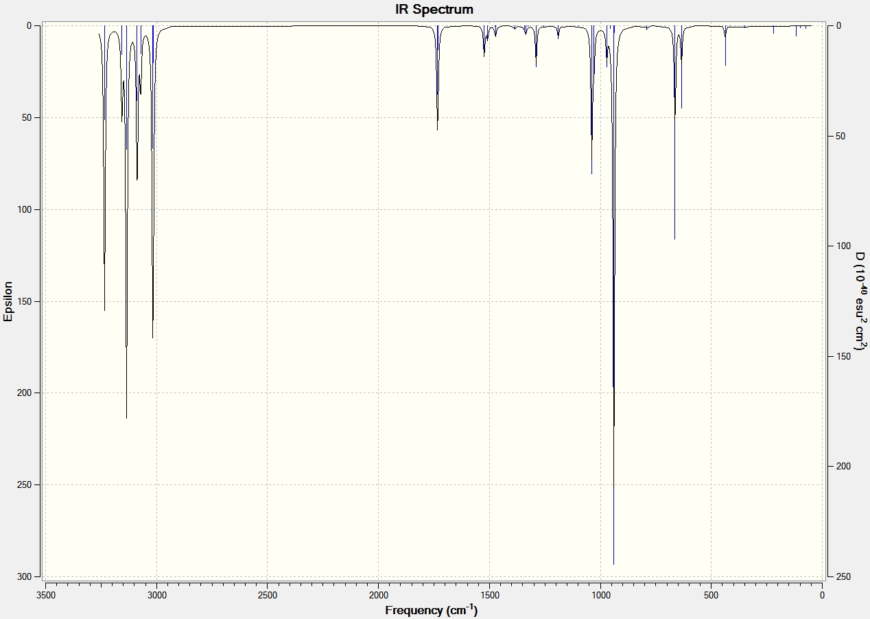
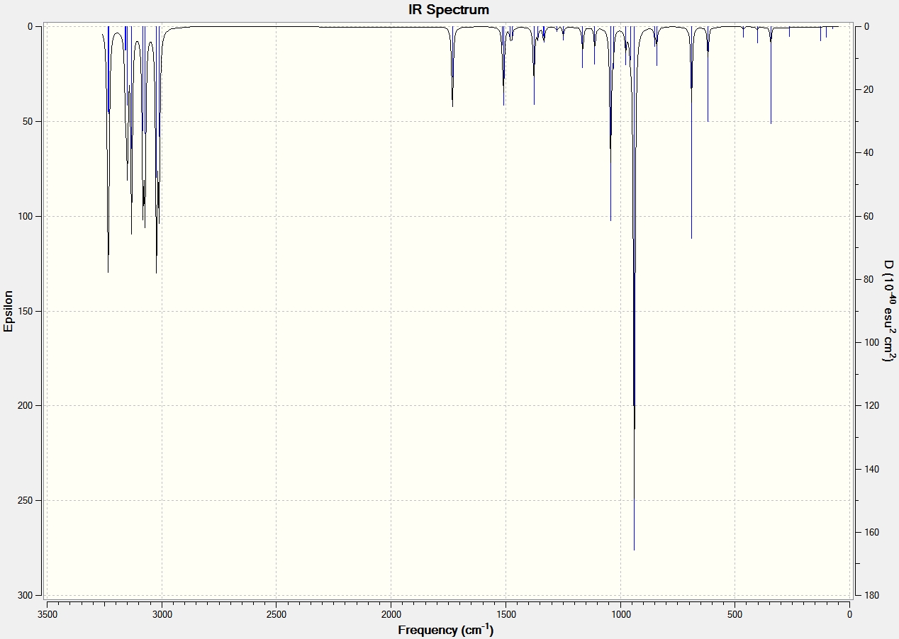
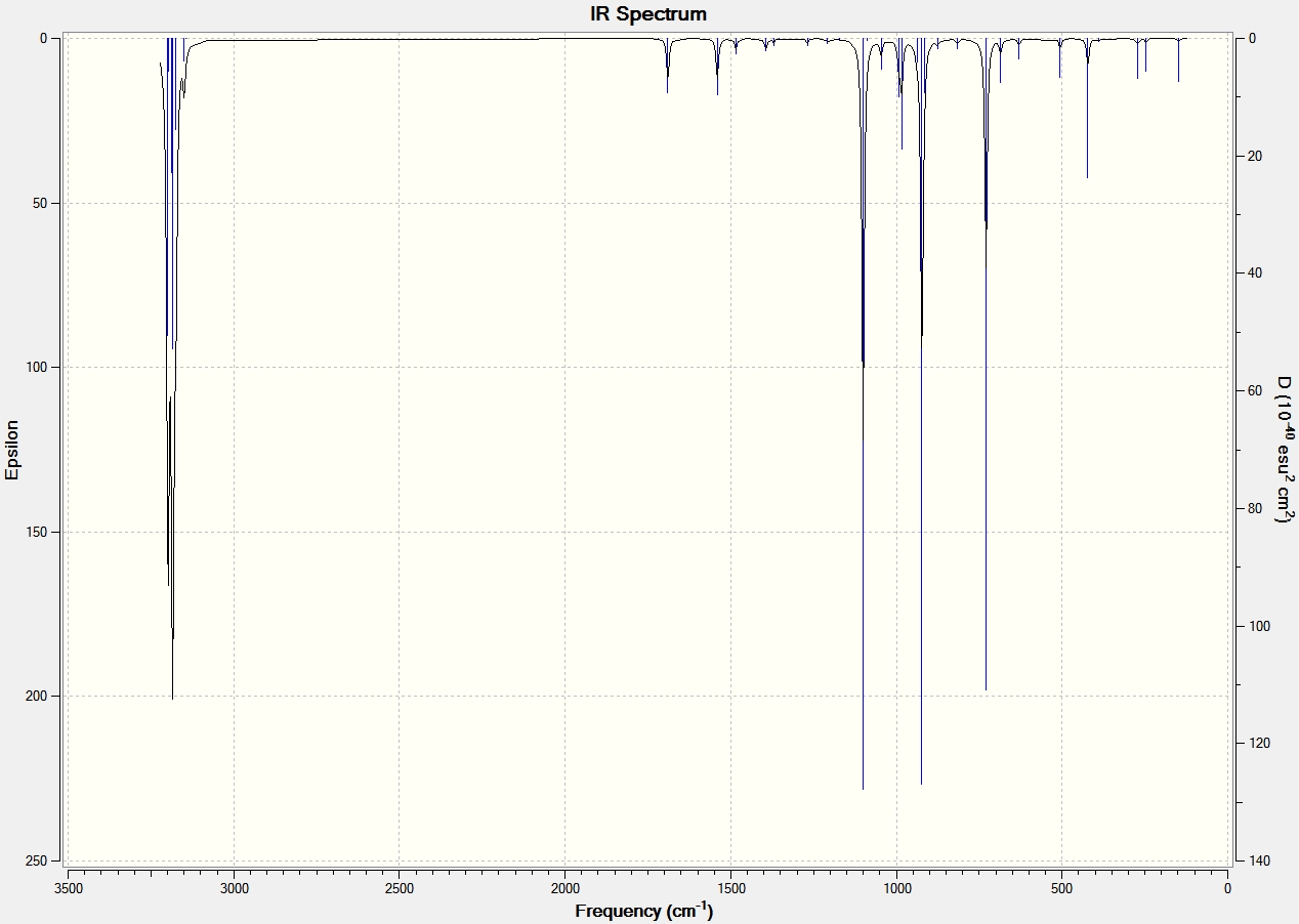
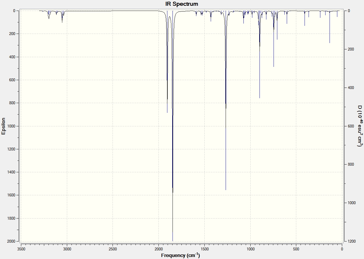
The two optimised reactant structures were both copied and pasted into a new window. They were then arranged to give a structure that was similar to what the transition structure would be expected to look like. The guess structure was then optimised using the frozen co-ordinate method since this has been seen to give reliable results in a convenient time frame. The semi empirical AM1 method was initially used and the terminal carbon distance was set to 2.00A. Once the first part of the frozen coordinate method was completed the terminal carbon bonds were unfrozen and set to derivative and the structure was optimised to a TS (Berny) via a Opt+Freq job. The calculation was sent to SCAN. The guess structure was also optimised via the frozen coordinate method using the DFT B3YLP/3-31G(d) method and basis set to give a comparison between the two methods. The table below gives a summary of the total energies of the transition state structures under both methods and also shows an animation of the imaginary vibrational stretches that demonstrates the transition state structures were found. This corresponds to the global maximum found due to the transition state. The IR spectrums can also be viewed by clicking on the appropriate link.
| Transition State Jmols | Method | Total Energy (Ha) | RMS Gradient | Animation | Frequency Stretche (cm-1) | Intensity | IR Spectrum |
|---|---|---|---|---|---|---|---|
| Transition State[38] | AM1 | 0.111654 | 0.000013 | Animation of Vibration | -956.29 | 5.63 | IR Spectrum |
| Transition State | AM1 | - | - | - | 147.89 | 0.2693 | - |
| Transition State[39] | DFT B3YLP/6-31G(d) | -234.54390 | 0.00005389 | Animation of Vibration | -525.23 | 5.83 | IR Spectrum |
| Transition State | DFT B3YLP/6-31G(d) | - | - | - | 135.44 | 0.7203 | - |
There is not a significant difference between the animations of the imaginary vibrations associated with the transition states under different methods. The animations show the concerted symmetrical motion of the two pairs of terminal carbons in the formation of the two new sigma bonds. This is as predicted since Diels alder reactions proceed via a concerted movement of electrons. The positive vibrational mode shows a non-concerted motion of electrons.
Molecular Orbital Analysis
The HOMO and LUMO of the transition state structures are shown below. The two methods were again contrasted to see if the level of theory of the calculations influenced the visual molecular orbitals.
| AM1 | DFT B3YLP/6-31G(d) | |
| LUMO |  |
 |
| HOMO |  |
 |
| HOMO-1 |  |
 |
| HOMO-2 |  |
 |
| HOMO-3 |  |
 |
| HOMO-4 |  |
 |
| HOMO-5 |  |
 |
| MO Energies |  |
 |
Focusing on the AM1 method molecular orbitals it can be seen that the LUMO is symmetric with respect to the plane of symmetry and the HOMO is antisymmetric. These molecular orbitals can be compared to the orbitals modelled for the reactants. It can be seen that the under the AM1 method, the LUMO of ethene and the HOMO of cis butadiene contribute to the transitions state HOMO. The HOMO of ethene and the LUMO of cis butadiene are the molecular orbitals contributing to the LUMO of the transition state.The HOMO of one reactant interacts with the LUMO of the other reactant, hence the reaction is allowed.
Whilst carrying out the molecular orbital analysis it was interesting to see that the HOMO of the transitions state was symmetric for the DFT B3LYP/6-31G(d) method but antisymmetric for the AM1 method. Therefore the HOMO-1 MO was viewed and an interesting result was seen. It seems that the HOMO and HOMO-1 have swapped for the different methods and this can be explained by looking at the relative energies of the orbitals. The HOMO and HOMO-1 are nearly degenerate in energy and therefore reorder depending on the method used. The other HOMO orbitals were also compared and it seems that degenerate pairs of molecular orbitals have also reordered. The difference in the molecular orbital shapes between the two methods also increases as the energy becomes more negative, suggesting that the electronic interaction used in the more sophisticated method influences the shape and delocalisation of the molecular orbitals more for the lower molecular orbitals.
The bond lengths in the transition states were measured and are tabulated below:
Bond Lengths of Transition States| Method | Point Group | Forming C-C (A) | Diene C=C (A) | Diene C-C (A) | Ethene C=C (A) |
|---|---|---|---|---|---|
| AM1 | cs | 2.11 | 1.38 | 1.40 | 1.38 |
| DFT B3YLP/6-31G(d) | cs | 2.27 | 1.38 | 1.41 | 1.39 |
The majority of the bond lengths are similar between the two methods used to calculate the transition structures. The main difference is the forming C-C bond difference. It is longer in the DFT B3YLP/6-31G(d) method. The Van der Waals radius is 1.70A for carbon so the expected distance between two non bonded carbons would approximate to double this at 3.40A[40]. The values predicted for the forming C-C bond are approximately half way between this distance value and the distance value of the C-C single bond. This insinuates that a bond would form between the terminal carbons to form the new sigma bond.
The literature values for the C=C bonds and C-C bonds are 1.33A and 1.53A respectively[41]. The C=C predicted bonds are slightly longer than this and the C-C bonds are shorter. This is because the results are based on the transition state structure and not the product structure.
Cyclohexa-1,3-diene and Maleic Anhydride Optimisation
The reaction between Cyclohexa-1,3-diene and Maleic Anhydride will now be investigated. This is another example of a Diels Alder reaction which can give two different stereospecific products depending on the conditions. The reaction yields entirely the endo product [42] which is surprising since the exo product is the more stable of the two. The exo product is more thermodynamically stable because there is less steric hindrance with the bulky anhydride ring and the carbon-carbon double bond.
The reaction demonstrates the effect of the endo rule where under kinetic and irreversible conditions it dominates. It is preferred since there is a favourable bonding interaction between the developing π bond on the back of the diene and the carbonyl groups on the dienophile[43]. The reaction scheme can be seen below and shows the mechanism for the 4s +2s cycloaddition.

First the reactants’ geometries were optimised under the two methods – Semi empirical AM1 and DFT B3YLP/6-31G(d). The reactants were drawn in GaussView and then the calculations were sent to SCAN. The total energies and point groups of the two reactants under different methods are summarised in the table below: The RMS gradient values are all very close to zero suggesting that a minimum energy structure was found.
Energies of the Reactants| Reactant | Method | Total Energy (Ha) | RMS Gradient | Point Group |
|---|---|---|---|---|
| Maleic Anhydirde[44] | AM1 | -0.121824 | 0.00005612 | C2v |
| Maleic Anhydirde[45] | DFT B3YLP/6-31G(d) | -379.28954 | 0.00000636 | C2v |
| Cyclohexa-1,3-diene[46] | AM1 | 0.02771 | 0.00000807 | C2 |
| Cyclohexa-1,3-diene[47] | DFT B3YLP/6-31G(d) | -233.41894 | 0.00003103 | C2 |
Molecular Orbital Analysis
The reactants molecular orbitals were also viewed and are shown below. The molecular orbitals are different for the different methods used and this is because the methods take into account different parameters in the calculations. The DFT B3YLP/6-31G(d) method considers more electronic interactions and takes into account delocalization or diffusion of the electrons in the bonds. The semi empirical method is based on the Hartree Fock theory, but makes many approximations and uses parameters from empirical data. This explains the different shapes of the Mos.
| Method | HOMO | LUMO |
| AM1 |  |
 |
| DFT B3YLP/6-31G(d) |  |
 |
| Method | HOMO | LUMO |
| AM1 |  |
 |
| DFT B3YLP/6-31G(d) |  |
 |
For AM1:
The cylcohexadiene HOMO is antisymmetric with respect to the plane of symmetry and the LUMO is symmetric.
The maleic anhydride HOMO is symmetric with respect to the plane of symmetry and the LUMO is anti symmetric
For DFT B3YLP/6-31G(d):
The cylcohexadiene HOMO is antisymmetric with respect to the plane of symmetry and the LUMO is symmetric.
The maleic anhydride HOMO is antisymmetric with respect to the plane of symmetry and the LUMO is also antisymmetric.
Transition State Optimisation
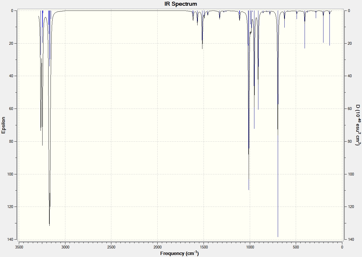
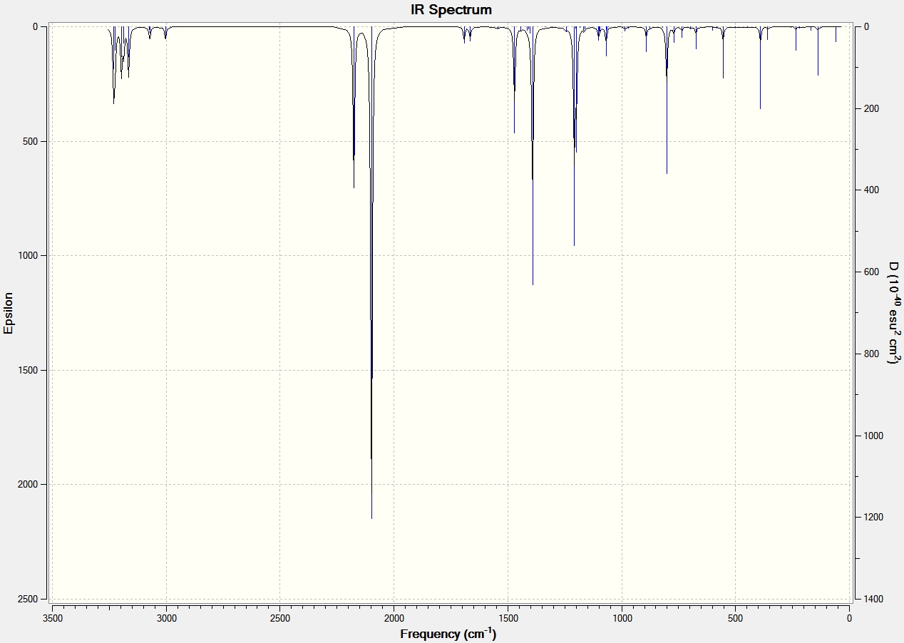
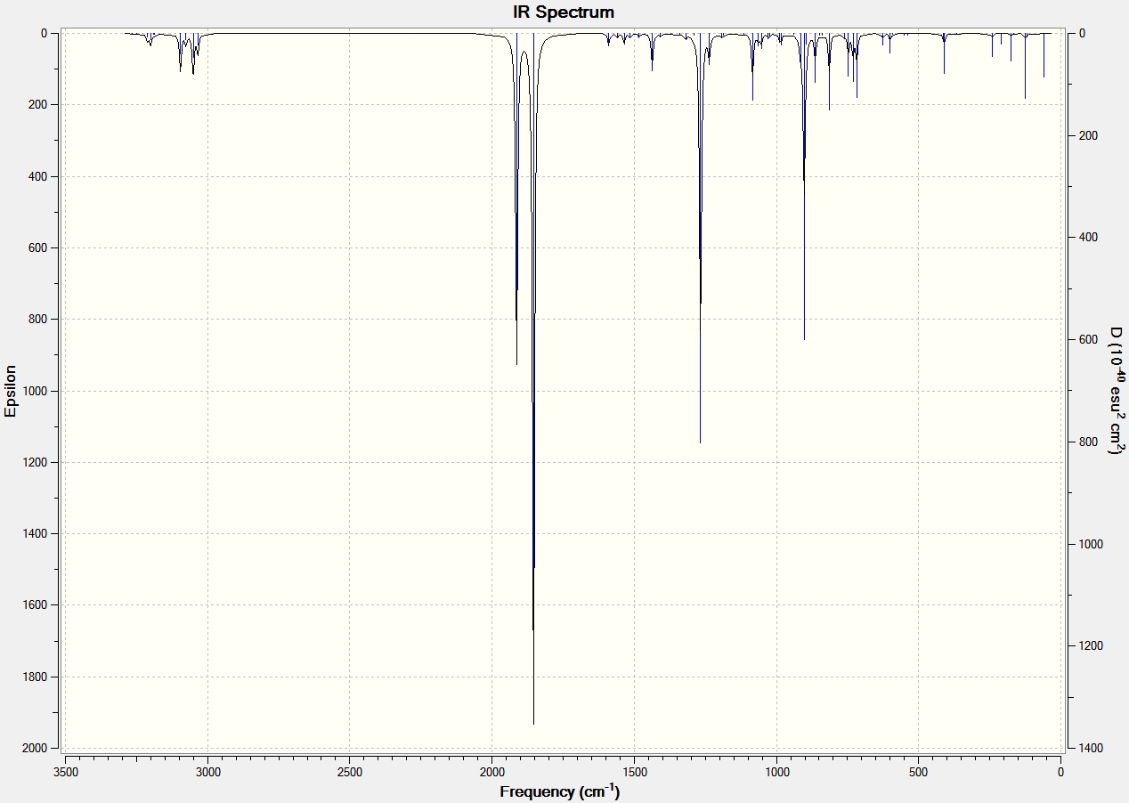
The two optimised reactants were copied into a new window and arranged again to the guess Exo transtition structure. The frozen coordinate method was then used to optimised the guess structure under the semi empirical AM1 method. First the bond distance between the terminal carbons was set to 2.10A and the frozen structure was optmised to a minimum. The calculation was sent to SCAN. The completed job was opened and the bonds were unfrozen and changed to ‘derivative’ instead. The structure was then optimised to a TS(Berny) in a Opt+Freq calculation. The calculation was sent to SCAN. The process was repeated for the Endo transition state structure and for the DFT B3YLP/6-31G(d) method and basis set. The results from the optimisations are shown in the table below. The imaginary vibrational mode can be animated and the IR spectrum can be viewed by clicking on the appropriate links.
| Transition State Jmols | Method | Total Energy (Ha) | RMS Gradient | Animation | Frequency Stretche (cm-1) | Intensity | IR Spectrum |
|---|---|---|---|---|---|---|---|
| Exo Transition State[48] | AM1 | -0.050420 | 0.0000126 | Animation of Vibration | -812.12 | 96.97 | IR Spectrum |
| Exo | AM1 | - | - | - | 60.86 | 0.5527 | - |
| Exo Transition State[49] | DFT B3YLP/6-31G(d) | -612.67931 | 0.0000075 | Animation of Vibration | -448.52 | 5.5097 | IR Spectrum |
| Exo | DFT B3YLP/6-31G(d) | - | - | - | 53.19 | 0.4094 | - |
| Endo Transition State[50] | AM1 | -0.05150 | 0.0000471 | Animation of Vibration | -806.82 | 71.31 | IR Spectrum |
| Endo | AM1 | - | - | - | 62.60 | 1.5325 | - |
| Endo Transition State[51] | DFT B3YLP/6-31G(d) | -612.68340 | 0.0000187 | Animation of Vibration | -446.95 | 1.45 | IR Spectrum |
| Endo | DFT B3YLP/6-31G(d) | - | - | - | 59.60 | 1.2848 | - |
The animations of the imaginary vibrational modes show the formation of the two new sigma bonds in a concerted manner, as expected from theory. This negative stretching frequency shows that a transition state was found. From both methods it can be seen that the Endo transition state is lower in energy than the Exo. The exo and endo transition state structures can be viewed by clicking on the appropriate link. It can be seen that there is no difference between the structures under the different methods with different levels of theory.
Molecular Orbital Analysis
The molecular orbitals of the semi empirical AM1 method were viewed and are shown below for the exo and endo transition state structures:
| EXO | ENDO | |
| LUMO+1 |  |
 |
| LUMO+1 Side View |  |
 |
| LUMO |  |
 |
| HOMO |  |
 |
| HOMO-1 |  |
 |
| MO Energies |  |
 |
It can be seen that for the Exo transition state structure:
The LUMO +1 is symmetric,
The LUMO is antisymmetric,
The HOMO is antisymmetric,
The HOMO-1 is symmetric,
with respect to the plane of symmetry
For the Endo transition state structure:
The LUMO +1 is symmetric,
The LUMO is antisymmetric,
The HOMO is antisymmetric,
The HOMO-1 is symmetric,
with respect to the plane of symmetry
By looking at the molecular orbitals of the reactants it is possible to see which reactant molecular orbitals contribute to the molecular orbitals of the transition state:
The HOMO of maleic anhydride and the LUMO of cyclohexadiene contribute to the Exo LUMO+1
The LUMO of maleic anhydride and the HOMO of cyclohexadiene contribute to the Exo LUMO
The LUMO of maleic anhydride and the HOMO of cyclohexadiene contribute to the Exo HOMO
The HOMO of maleic anhydride and the LUMO of cyclohexadiene contribute to the Exo HOMO-1
The HOMO of maleic anhydride and the LUMO of cyclohexadiene contribute to the Endo LUMO+1
The LUMO of maleic anhydride and the HOMO of cyclohexadiene contribute to the Endo LUMO
The LUMO of maleic anhydride and the HOMO of cyclohexadiene contribute to the Endo HOMO
The HOMO of maleic anhydride and the LUMO of cyclohexadiene contribute to the Endo HOMO-1
The LUMO+1 orbitals were also viewed from the side to show the favourable secoundary interaction. It can be seen that this interaction is greater for the Endo transition state structure than the exo. The Endo transition state has a through space bonding interaction between the dienophile and the developing π bond at the back of the diene. This stabilising interaction is due to the correct symmetry of HOMO and LUMO frontier orbitals.
The bond distances between atoms were measured on GuassView and the distances tabulated below: It can be seen that all the bond lengths between the two methods are relatively similar, with the only major difference being the forming C-C bond. This difference is due to the different parameters associated with the different levels of theory in the calculations. By comparing the exo and endo forming C-C bonds it can be seen that the endo has a slightly shorter distance suggesting that the endo product is more likely to form.
Bond Lengths of Transition States| Transition State | Method | Forming C-C (A) | Cyclodiene C=C (A) | Cyclodiene C-C (A) | Anhydride C=O (A) | Anhydride C=C |
|---|---|---|---|---|---|---|
| EXO | AM1 | 2.17 | 1.39 | 1.40 | 1.22 | 1.41 |
| EXO | DFT B3YLP/6-31G(d) | 2.29 | 1.39 | 1.40 | 1.20 | 1.40 |
| ENDO | AM1 | 2.16 | 1.39 | 1.40 | 1.22 | 1.41 |
| ENDO | DFT B3YLP/6-31G(d) | 2.27 | 1.39 | 1.40 | 1.20 | 1.39 |
IRC Analysis
The IRC was calculated for the two trasition states under the AM1 method. The force constant was set to be computed in both directions. The exo transition state terminated in 74 steps, and the endo in 76 steps. Both IRC plots show that the initial geometries of the two reactants pass over a transition state (where the RMS gradient reaches zero) and then drop to a low energy product. The final structures can be viewed as Jmols, and show a structure resembling that of the expected product geometries.
| EXO[52] |  |
 |
| ENDO[53] |  |
 |
Conclusion
This module has demonstrated how useful computational chemistry can be in predicting transition state structures. The freeze co-ordinate method has been very useful in optimising the structures and is not extremely time consuming.
Throughout the module a comparison has been made between the different methods used in calculations. It is important to consider the parameters that they take account of when chosing the method to use. The AM1 semi empirical method has been extremely useful since it has given reliable results and has not been time consuming. The more sophisticated DFT B3YLP/6-31G(d) method was much more time consuming but also gave reliable predictions and took account of more interactions.
The frequency analysis has been useful in proving that a transition state structure has been found, since an imaginary vibration is seen.
The IRC calculation can be carried out rapidly and the results give a clear conclusion of whether a transition state has formed.
Overall computational chemistry can be used as a very powerful tool to anaylse the reactants, transition states and products in a reaction.
References
- ↑ O. Wiest et al., J. Am. Chem. Soc., 116, 1994, pp 10336
- ↑ http://hdl.handle.net/10042/to-12258
- ↑ http://hdl.handle.net/10042/to-12259
- ↑ http://hdl.handle.net/10042/to-12265
- ↑ http://hdl.handle.net/10042/to-12267
- ↑ http://hdl.handle.net/10042/to-12267
- ↑ http://hdl.handle.net/10042/to-12268
- ↑ http://hdl.handle.net/10042/to-12268
- ↑ http://hdl.handle.net/10042/to-12266
- ↑ http://hdl.handle.net/10042/to-12266
- ↑ J. Coates, Encyclopaedia of Analytical Chemistry, R. A. Meyers (Ed.), 2000, pp 10815 - 10831
- ↑ 3rd Year Computational Chemistry Online Lab Manual, Module 3, 2011
- ↑ http://hdl.handle.net/10042/to-12269
- ↑ http://hdl.handle.net/10042/to-12270
- ↑ http://hdl.handle.net/10042/to-12271
- ↑ http://hdl.handle.net/10042/to-12320
- ↑ http://hdl.handle.net/10042/to-12319
- ↑ http://hdl.handle.net/10042/to-12318
- ↑ http://hdl.handle.net/10042/to-12317
- ↑ http://hdl.handle.net/10042/to-12315
- ↑ http://hdl.handle.net/10042/to-12316
- ↑ http://hdl.handle.net/10042/to-12314
- ↑ http://hdl.handle.net/10042/to-12313
- ↑ http://hdl.handle.net/10042/to-12312
- ↑ http://hdl.handle.net/10042/to-12311
- ↑ http://hdl.handle.net/10042/to-12310
- ↑ http://hdl.handle.net/10042/to-12319
- ↑ http://hdl.handle.net/10042/to-12319
- ↑ http://hdl.handle.net/10042/to-12325
- ↑ http://hdl.handle.net/10042/to-12325
- ↑ http://hdl.handle.net/10042/to-12321
- ↑ http://hdl.handle.net/10042/to-12321
- ↑ http://hdl.handle.net/10042/to-12324
- ↑ http://hdl.handle.net/10042/to-12324
- ↑ J. Clayden et al., Organic Chemistry, Oxford University Press, United States, 2001, pp 905 - 918
- ↑ http://hdl.handle.net/10042/to-12328
- ↑ http://hdl.handle.net/10042/to-12327
- ↑ http://hdl.handle.net/10042/to-12333
- ↑ http://hdl.handle.net/10042/to-12327
- ↑ A. Bondi et al., J. Phys. Chem., 68 (3), 1964, pp 441 - 451
- ↑ D. R. Lide, Tetrahedron, 17, 1962, pp 125 - 134
- ↑ Clayden
- ↑ Clayden
- ↑ http://hdl.handle.net/10042/to-12345
- ↑ http://hdl.handle.net/10042/to-12348
- ↑ http://hdl.handle.net/10042/to-12346
- ↑ http://hdl.handle.net/10042/to-12347
- ↑ http://hdl.handle.net/10042/to-123999
- ↑ FREQ http://hdl.handle.net/10042/to-12395
- ↑ http://hdl.handle.net/10042/to-12393
- ↑ http://hdl.handle.net/10042/to-12396
- ↑ http://hdl.handle.net/10042/to-12526
- ↑ http://hdl.handle.net/10042/to-12527