
Rep:Mod:gf609mod2
Computational Inorganic Chemistry
Introduction
Computational chemistry will be used to investigate the bonding and structural characteristics in inorganic compounds and complexes which can be found from the analysis of the electron density between atoms. An advantage that computational chemistry has over experimental studies is that it is capable of characterising the location of activated complexes and transition states as well as being able to distinguish between the energy of stable conformers. Properties such as NMR spectra, IR spectra and dipole moments can also be calculated.
Before analysis, optimisation of all molecules is carried out. In an optimisation the SCF part of the calculation is where the position of the nuclei are assumed (represented as R1). The Schrödinger equation is then solved for the electron density rho(R1) and energy E(R1). Next the OPT part of the calculations is solved for the position of the nuclei. Here the nuclei are moved to different positions and the SFC cycle repeated for different geometries. This gives out a series of different energies that are reliant upon the different positions of the nuclei and electrons and is known as a potential energy surface. The geometry that gives the lowest energy is the optimised geometry[1].
In a potential energy surface the minimum point is the stable state and equilibrium position. This is where the electrons and nuclei have no forces trying to shift their positions. At this minimum point the first derivative (gradient) of the curve is zero. However maximum points and points of inflection can also have first derivatives of zero. It is therefore necessary to take the second derivative of the curve. A minimum point will have a positive second derivative value, and a maximum point will have a negative one.
In solving the Schrödinger equation the approximations are determined by the BLYP method, and the accuracy determined by the 3-21G basis set. Although this basis set gives low accuracy, it is chosen because calculations can be performed quickly. An example of the power of computational chemistry can be read [2] demonstrating how computational chemistry was used in the production of polymers to find cheaper alloys that selectively remove ethyne from a stream of ethane.
BH3
Optimisation Analysis of BH3
Gaussview 5.0 was used to create a molecule of BH3 with initial bond lengths set to 1.5A. Gaussian was then used to optimise the molecules energy. The DFT B3LYP method and the 3-21G basis set were used. The summary of the optimisation to give the optimised geometry is shown in the table below. The gradient is close to zero and indicates that optimisation was completed.

The images below show the bond distance and bond angle of the optimised H-B-H bond - 1.19Å and 120° respectively. These are identical to those of literature of 1.19Å [3] and 120°[4]. This is because BH3 is a very simple molecule with few electrons, therefore the assumptions in the calculations do not affect the optimised structure significantly. It is therefore close to that of the experimental structure.
 |
 |
Below shows the set of forces and displacements that show that the job has converged, it indicates that for a small displacement, the energy of the molecule does not change.
 Item        	    Value  	Threshold  Converged?
 Maximum Force       	   0.000413     0.000450        YES
 RMS     Force             0.000271     0.000300    	YES
 Maximum Displacement      0.001610     0.001800        YES
 RMS     Displacement      0.001054     0.001200        YES
 Predicted change in Energy=-1.071764D-06
 Optimization completed.
 -- Stationary point found.
----------------------------
                           !   Optimized Parameters   !
                           ! (Angstroms and Degrees)  !
 --------------------------                            --------------------------
 ! Name  Definition              Value          Derivative Info.                !
 --------------------------------------------------------------------------------
 ! R1    R(1,2)                  1.1935         -DE/DX =    0.0004              !
 ! R2    R(1,3)                  1.1935         -DE/DX =    0.0004              !
 ! R3    R(1,4)                  1.1935         -DE/DX =    0.0004              !
 ! A1    A(2,1,3)              120.0            -DE/DX =    0.0                 !
 ! A2    A(2,1,4)              120.0            -DE/DX =    0.0                 !
 ! A3    A(3,1,4)              120.0            -DE/DX =    0.0                 !
 ! D1    D(2,1,4,3)            180.0            -DE/DX =    0.0                 !
 --------------------------------------------------------------------------------
The first optimisation graph below shows the energy of the BH3 molecule throughout the optimisation. A minimum optimised energy value is reached after 4 iterations. The second graph shows the RMS gradient at each step of optimisation which reaches a value towards zero.


The animation of the optimisation steps is shown below. It shows the position of the nuclei at each step. The final structure (4th iteration) corresponds to the most negative energy and smallest gradient and therefore the optimized geometry.

NBO Analysis of BH3
The log file of the calculation sent to SCAN was opened in Gaussview to view the charge distribution of the BH3 molecule. The images below show that the central boron atom is highly positively charged as expected since it is lewis deficient. The hydrogen atoms are red and negatively charged. The NBO charges for the boron and hydrogen are 0.3316 and -0.1105 respectively, which can be found from the summary of natural population analysis. All hydrogen atoms have the same charge since the molecule is symmetrical and the total charge of the hydrogen atoms cancels out the positive charge of the boron atom to give a neutral molecule overall.

 Summary of Natural Population Analysis:

                                       Natural Population
                Natural  -----------------------------------------------
    Atom  No    Charge         Core      Valence    Rydberg      Total
 -----------------------------------------------------------------------
      B    1    0.33161      1.99903     2.66935    0.00000     4.66839
      H    2   -0.11054      0.00000     1.11021    0.00032     1.11054
      H    3   -0.11054      0.00000     1.11022    0.00032     1.11054
      H    4   -0.11054      0.00000     1.11022    0.00032     1.11054
 =======================================================================
   * Total *    0.00000      1.99903     6.00000    0.00097     8.00000
The nature of the bonds in the molecule can be seen below. The first three orbitals show the relative electronic contribution in a bond from each atom either end of the bond. It can be seen that in each BH bond, the boron contributes 44.48% of the electron density, and the hydrogen contributes 55.52%. This is as expected since the hydrogen is more electronegative and is therefore a greater contributor of electron density to the bond.
The hybridisation of the bonds can also be seen from the data below. It is clear that the ratio of s and p character in the bond is 1:2 and suggesting a sp2 hybridised bond. This is as expected since the H-B-H bond angle is 120o and the point group of the molecule is D3h.
The fourth orbital is the boron 1s atomic orbital and it therefore has 100% s character. Orbital 5 should be the lone pair p orbital and is starred since it is unoccupied. However the data below shows that it has 100% s character and not 100% p character as expected. This is an error in the data could be due to the method in which the calculation was carried out.
(Occupancy)   Bond orbital/ Coefficients/ Hybrids
---------------------------------------------------------------------------------
     1. (1.99853) BD ( 1) B   1 - H   2
                ( 44.48%)   0.6669* B   1 s( 33.33%)p 2.00( 66.67%)
                                            0.0000  0.5774  0.0000  0.0000  0.0000
                                            0.8165  0.0000  0.0000  0.0000
                ( 55.52%)   0.7451* H   2 s(100.00%)
                                            1.0000  0.0000
     2. (1.99853) BD ( 1) B   1 - H   3
                ( 44.48%)   0.6669* B   1 s( 33.33%)p 2.00( 66.67%)
                                            0.0000  0.5774  0.0000  0.7071  0.0000
                                           -0.4082  0.0000  0.0000  0.0000
                ( 55.52%)   0.7451* H   3 s(100.00%)
                                            1.0000  0.0000
     3. (1.99853) BD ( 1) B   1 - H   4
                ( 44.48%)   0.6669* B   1 s( 33.33%)p 2.00( 66.67%)
                                            0.0000  0.5774  0.0000 -0.7071  0.0000
                                           -0.4082  0.0000  0.0000  0.0000
                ( 55.52%)   0.7451* H   4 s(100.00%)
                                            1.0000  0.0000
     4. (1.99903) CR ( 1) B   1           s(100.00%)
                                            1.0000  0.0000  0.0000  0.0000  0.0000
                                            0.0000  0.0000  0.0000  0.0000
     5. (0.00000) LP*( 1) B   1           s(100.00%)
Frequency Analysis
Guassian was used to calculate the frequency of the BH3 molecule. The summary is shown below. An IR spectrum was also computed from the vibrational analysis. All the frequencies calculated were positive showing that a global minimum was determined and that the optimisation of the molecule was successful. In the IR spectrum there are three peaks which is less than the six vibrations of the molecule . This can be explained by looking at the vibrational modes of each vibration (shown in the table below). The A1’ vibrational mode has no change in dipole moment since it is totally symmetric, it therefore has no peak. There is also a pair of E’ vibrational modes which are degenerate and so would only show one peak for the two vibrations.


Guassview was used to show the different modes of vibrations of the molecule with animation, and snap shots of these animations are shown in the table below with details of the description of the vibration. The frequencies were also compared to that of literature[5]. The symmetry label for each vibration was also determined since the point group of BH3 is D3h.
| Vibrational Mode | Vibrational Mode Diagram | Vibrational Mode Description | Vibrational Mode Intensity | Vibrational Mode Frequency (cm-1) | Literature Frequency (cm-1) |
|---|---|---|---|---|---|
| A2"' |  |
Hydrogens move together backwards and forwards - umbrella deformation | 92.87 | 1144.15 | 1147.5 |
| E' |  |
One hydrogen is still and the other two move symmetrically rocking - Symmetric B-H scissoring | 12.31 | 1203.64 | 1196.7 |
| E' |  |
All B-H bonds rock, one with greater magnitude than the others - Asymmetric B-H rock | 12.31 | 1203.64 | 1196.7 |
| A1' |  |
All B-H bonds symmetrically stretch, the bonds elongate together and then compress. B-H symmetric stretch | 0.00 | 2598.42 | 2503 |
| E' |  |
Two B-H bonds stretch symmetrically and the thrid stretches antisymmetrically - Asymmetric B-H stretch | 103.74 | 2737.44 | 2601.6 |
| E' | |
Two B-H bonds stretch asymmetrically and the third H remains static. Asymmetric B-H Stretch | 103.73 | 2737.44 | 2601.6 |
Molecular Orbitals in BH3
The energy of the optimised BH3 structure was calculated using additional keywords ‘pop=full’ to turn on the MO analysis. FULL NBO was selected and the same method and basis sets from the optimisation calculation were used. The job was sent to SCAN [6]. The calculation solves the electronic structure of the molecular and gives out quantitative molecular orbitals which can then be compared to the qualitative MO from a MO diagram.
The checkpoint file was opened in Gaussview and the MOs of BH3 were viewed. The HOMO is shown to be the fourth MO and the LUMO the fifth. A comparison between the calculated MOs and the MOs form the MO diagram is shown below. The MO diagram was created via the Linear Combination of Atomic Orbitals[7] approach. The two fragments of the BH3 molecule were drawn with the H3 fragment orbital drawn slightly lower in energy than the boron since the hydrogens are slightly more electronegative than the boron – 2.08 and 1.85 respectively [8]. Fragment orbitals of the same symmetry were combined and the electrons from each fragment orbital were added into the molecular orbitals (giving a total of 8 electrons). The HOMO and LUMO were then determined. The 1s atomic orbital of boron is not shown on the MO diagram since it is too low in energy. This is also seen form the calculated MO where it has a value of -6.73023 which is much lower than the rest of the MOs. It is difficult to evaluate the ordering of the 3a’ and the 2e’ orbitals in the MO diagram since when s-s interactions are stronger than s-p it is likely that the 3a’ would be higher, however the a1’ energy levels are usually lower than e’ making 3a1’ lower.


The MO diagram and the calculated MOs are very similar. BH3 is a simple molecule however a more complex molecule with more electrons would need more computing power for computational analysis.
The low frequencies were found and are shown below:
Low frequencies ---   -0.3716   -0.0098   -0.0018   37.2444   37.9574   37.9592
 Low frequencies --- 1146.0292 1204.8631 1204.8641
TlBr3
Optimisation Analysis of TlBr3
A more complex trigonal planar molecule, TlBr3, was created in Guassview. TlBr3 has 186 electrons which makes it more complicated than the BH3 molecule. The assumption made is that only the valence electrons dominate the bonding interactions and the other electrons are modelled by pseudo potentials. The optimised ground state structure was calculated in Guassian by first setting the point group to D3h and then using the DFT BYL3P method and LanL2DZ basis set which is a medium level basis set and considers pseudo potentials. This allows for a more accurate analysis of the molecule. The optimisation summary that calculated the optimised geometryis shown below, it shows a dipole moment close to 0 due to the highly symmetrical molecule:

The bond angle and the bond length of Br-Tl-Br was found to be 120o and 2.65 A respectively which is close to the literature values of 120 degrees[9] and 2.52 A [10]. The bond and angle measurements are shown below:
 |
 |
Below show the set of forces and displacements that show the job converged:
Item               Value     Threshold  Converged?
 Maximum Force            0.000002     0.000450     YES
 RMS     Force            0.000001     0.000300     YES
 Maximum Displacement     0.000022     0.001800     YES
 RMS     Displacement     0.000014     0.001200     YES
 Predicted change in Energy=-6.082811D-11
 Optimization completed.
    -- Stationary point found.
----------------------------
                           !   Optimized Parameters   !
                           ! (Angstroms and Degrees)  !
 --------------------------                            --------------------------
 ! Name  Definition              Value          Derivative Info.                !
 --------------------------------------------------------------------------------
 ! R1    R(1,2)                  2.651          -DE/DX =    0.0                 !
 ! R2    R(1,3)                  2.651          -DE/DX =    0.0                 !
 ! R3    R(1,4)                  2.651          -DE/DX =    0.0                 !
 ! A1    A(2,1,3)              120.0            -DE/DX =    0.0                 !
 ! A2    A(2,1,4)              120.0            -DE/DX =    0.0                 !
 ! A3    A(3,1,4)              120.0            -DE/DX =    0.0                 !
 ! D1    D(2,1,4,3)            180.0            -DE/DX =    0.0                 !
 --------------------------------------------------------------------------------
The RMS of 0.000014 is very close to zero showing that optimisation completed and the job converged. A minimum optimised energy value of -91.21812 is reached after 3 iterations. The graphs below show how the energy and the RMS gradient change throughout the optimisation of TlBr3:


The animation below shows the position of the nuclei at each optimisation step. The third iteration is the final optimised geometry which has the most negative energy and the smallest gradient.

Frequency Analysis
Guassian was used to calculate the frequency of the TlBr3 molecule. The summary is shown below. An IR spectrum was also computed from the vibrational analysis. Again all the frequencies calculated were positive showing that a global minimum was determined and that the optimisation of the molecule was successful. If the values were negative, a global maximum would be found which would be associated with the transition state and not the final optimised geometry.

In the IR spectrum there are three peaks which is less than the six vibrations of the molecule . This can be explained in the same way as the BH3 molecule by looking at the vibrational modes of each vibration (shown in the table below). The A1’ vibrational mode has no change in dipole moment since it is totally symmetric, therefore there is no peak associated with this vibration. There is also a pair of E’ vibrational modes which are degenerate and so would only show one peak for the two vibrations.

Guassview was used to show the animations of the different modes of vibrations, and snap shots of these animations are shown in the table below with details of the description of the vibration. The frequency values were compared to that of literature[11]. The symmetry label for each vibration was also determined since the point group of TlBr3 is D3h.
| Vibrational Mode | Vibrational Mode Diagram | Vibrational Mode Description | Vibrational Mode Intensity | Vibrational Mode Frequency (cm-1) | Literature Frequency (cm-1) |
|---|---|---|---|---|---|
| E' |  |
Two Tl-Br bonds rock symmetrically whilst the other Br remains static - symmetric Tl-Br Scissoring | 3.69 | 46.43 | 47 |
| E' |  |
All Tl-Br bonds rock, one with a greater magnitude than the others - Asymmetric Tl-Br rock | 3.69 | 46.43 | 47 |
| A2" |  |
All Br move together backwards and forwards - umbrella deformation | 5.85 | 52.14 | 63 |
| A1' |  |
All Tl-Br bonds symmetrically stretch, the bonds elongate together and then compress. Tl-Br symmetric stretch | 0.00 | 165.27 | 185 |
| E' |  |
Two Tl-Br bonds stretch asymmetrically and the third H remains static. Asymmetric Tl-Br Stretch | 25.48 | 210.69 | 203 |
| E' |  |
Two Tl-Br bonds stretch symmetrically and the thrid stretches antisymmetrically - Asymmetric Tl-Br stretch | 25.48 | 210.69 | 203 |
The low frequencies for TlBr3 are shown below:
Low frequencies ---   -0.3716   -0.0098   -0.0018   37.2444   37.9574   37.9592
 Low frequencies --- 1146.0292 1204.8631 1204.8641
It must be noted that GaussView has a set of pre-defined bond lengths and therefore occasionally bonds that do exist but are slightly longer than the defined values are not drawn in the molecule. It is therefore necessary to use chemical intuition when analysing optimised molecules since computational chemistry can only give a quantitative analysis where the calculations have had to use methods with parameters in place. Computational chemistry cannot qualitatively analyse a bond and this is what must be remembered when carrying out calculations. Bonds can be loosely categorised into three types of bonds; ionic, covalent and metallic. An ionic bond is the electrostatic attraction between two atoms of opposite charge. A covalent bond is a chemical bond where a there is an overlap between valence molecular orbitals (ie electrons are shared between atoms) in a molecule. A metallic bond is where fixed positively charged nuclei are held together by a ‘sea’ of delocalised electrons. This delocalisation allows electronic conduction.
Isomers of Mo(CO)4L2
Introduction
In second year laboratory the cis and trans isomers of the Mo(CO)4(PPh3)2 complex were studied and their IR spectrums analysed. It was seen that the cis- complex had four stretching frequencies and the trans only one. In this section two isomers of the Mo(CO)4L2 complex were modelled using computational chemistry to find the relative thermal stability and the spectral characteristics of both. The ligand used is different to that studied in second year lab and is the -PCl3 ligand instead of the -PPh3 ligand. The PPh3 ligand has a much larger number of electrons compared to Pcl3 and is therefore too complex to calculate with the computing power available. Similar results should be seen however, since the chlorine atoms contribute to bonding and sterics in a similar way to the phenyl group.
Optimisation Analysis of Mo(CO)4(PCl3)2
The two isomers were created in GaussView and then loosely optimised using the B3LYP method and the LANL2MB basis set. “opt=loose” was written into the additional keywords. These are low level basis set and pseudo-potential settings and were used to calculate the initial and rough geometry of the complexes. The input file was sent to SCAN [12] [13].
The geometry from this low level optimisation was tweaked manually to improve the dihedral angles to a more favourable geometry. For the cis isomer, the chlorine groups on one of the phosphorus atoms were rotated so that one of the chlorine atoms pointed up parallel to the axial bond, and the chlorines on the other phosphorus atom were rotated so that one chlorine pointed down. For the trans isomer, the PCl3 groups were eclipsed with one chlorine on each phosphorus pointing down. These tweaked structures were then sent to SCAN [14] [15] for further optimisation using the B3LYP method and the LANL2DZ (double zeta) pseudo-potential. These are far better basis sets and pseudo potential settings, therefore a tighter convergence is required. So the additional keywords “int=ultranfine scf=conver=9” were entered to increase electronic convergence.
 |
The geometry from this optimisation was then further optimised by adding the dAO functions which should be taken into account since phosphorus is capable of hypervalency. The output file from the previous optimisation was opened in wordpad and extrabasis settings were added. The file was sent to SCAN [16] [17]. The summaries of the optimisations are shown below. It can be seen that the trans is ever so slightly more thermodynamically stable since it has a lower energy when taking the dAOs into account. This is different to the results from the second optimisation above where it is suggested that the cis is thermodynamically more stable. It is interesting to see how the change in basis sets can alter this conclusion. It must be noted that there is a rough error of 0.0038 Ha in the energies calculated above. The conclusion drawn from the extrabasis optimisation where the trans is more thermodynamically stable is the same conclusion found from experimental analysis in second year lab. Here it was found that at higher temperatures the cis isomer isomerises to the trans isomer, and once the initial energy barrier is overcome, the isomer exists as the trans form of the complex. The decomposition temperatures of 148˚C -150˚C[18] for the cis and 163˚C-168˚C[19] for the trans also supports this conclusion. The explanation for the trans isomer being more thermodynamically favoured is due to the position of the bulky PCl3 ligands which are placed as far apart as possible in the octahedral complex, relieving steric hindrance found in the cis isomer. A way of making the cis isomer more thermodynamically stable would be to change the ligand to make the interactions between the ligands favourable. For example if the chlorine atoms on the phosphorus were replaced with groups capable of hydrogen bonding, the cis form would most likely be more stable due to strong favourable interactions between a hydrogen atom (attached to an electronegative atom) and a highly electronegative atom. Hence simply changing all the Cl atoms to OH groups would change the stability of the isomers relative to each other.
 |
The optimised geometries taking account of the d atomic orbital contribution can be viewed in the Jmols below. The bond lengths of the final optimised geometries were measured and compared to literature values[20][21] in the table below as another way of ensuring the calculations were completed correctly:
| Cis Bond Lengths (angstroms) | Literature Bond Length (angstroms) | Trans Bond Lengths (angstroms) | Literature Bond Length (angstroms) | |
|---|---|---|---|---|
| Mo-C Bond | 2.05 | 2.01 | 2.06 | 1.87 |
| Mo-P Bond | 2.48 | 2.58 | 2.42 | 2.37 |
| C-O Bond | 1.17 | 1.15 | 1.16 | 1.15 |
| P-Cl Bond | 2.12 | 1.83 | 2.12 | - |
Literature values for the Mo complex undergoing investigation was difficult to find, therefore the trans and cis structures were compared to complexes which were deemed to be similar; trans – Cr(CO)4(PPh3)2 and cis-Mo(CO)4(PPh3)2 respectively. From the table it can be seen that all the bond lengths are relavtively close to that of literature. The bond that shows the greatest difference to literature is the cis P-Cl bond. This may be due to the fact we are comparing a P-Cl bond to a literature P-Ph bond, however an alternative reason for the difference may be that the orbital interactions that were considered in the calculation were not complex enough to calculate an accurate bond length. This bond length was compared to the bond length after the second optimisation to see if taking the dAOs into consideration made any difference to this particular value. The bond length was .for the 2.24A P-Cl bond which was ever further from the literature value. This demonstrates that using a basis set which considers d-orbital interactions calculated more favourable Mo-P interaction which allowed for better electron donation from the P to the Cl forming a stronger and therefore shorter bond.
When comparing the two isomers, all but one value are relatively similar and within 0.01 Å of each other. The bond length that differs is the Mo-P bond length, where in the cis isomer it is slightly longer than the trans. This suggests that the cis bond is weaker than the trans and can be explained by the fact that in the cis complex, the two bulky ligands are in close proximity and therefore must lengthen the bond to reduce steric hindrance. The cis complex configuration is therefore the less thermodynamically stable of the two due to the unfavourable interaction between the bulky groups.
The results also suggest that the trans effect occurs slightly between the carbonyl ligand and the P ligand in the cis-isomer. Here, the P is capable of donating electrons into the metal centre which increases the back bonding from the metal to the carbonyl ligand. The results show that in the cis isomer the Mo-C bond is slightly shorter and therefore stronger than the trans isomer (due to backbonding) and that the C-O bond is slightly longer and therefore weaker (also explained by backbonding).
Frequency Analysis of Mo(CO)4(PCl3)2
To investigate the spectral characteristics of the isomers, the frequency of the complexes were calculated using the extrabasis optimised geometries. The LANL2DZ basis set was used again with the additional key words “int=ultranfine scf=conver=9”. It was necessary to go into the output file of the optimised geometries to check that the input file sent to SCAN had the correct extrabasis settings for the frequency calculation [22][23]. The frequencies below are focused on the carbonyl region and the vibrational modes of the Mo-P bond (lower frequencies). The point group of the cis isomer is C2v and the trans is D4h. Using these poitn groups, each vibrational mode was determined as shown below::
| Vibrational Mode | Vibrational Mode Diagram | Vibrational Mode Description | Vibrational Mode Intensity | Vibrational Mode Frequency (cm-1) | Literature Frequency (cm-1) |
|---|---|---|---|---|---|
| - |  |
PCl3 groups rotate symmetrically back and forth | 0.0037 | 11.21 | |
| - |  |
PCl3 groups rotate asymmetrically back and forth | 0.0323 | 19.04 | |
| B2' |  |
Asymmetric stretching of the carbonyl groups trans to the PCl3 | 753.84 | 1946.66 | 1869 |
| B2 |  |
Asymmetric stretching of carbonyl groups trans to each other | 1501.79 | 1949.80 | 1896 |
| A1' |  |
All carbonyl groups stretch. Two pairs of carbonyls asymmetrically stretch with respect to one another | 615.61 | 1959.20 | 1924 |
| A1' |  |
All carbonyl groups symmetrically stretch | 577.83 | 2024.00 | 2026 |
| Vibrational Mode | Vibrational Mode Diagram | Vibrational Mode Description | Vibrational Mode Intensity | Vibrational Mode Frequency (cm-1) | Literature Frequency (cm-1) |
|---|---|---|---|---|---|
| - | PCl3 groups rotate symmetrically back and forth | 0.0547 | 4.45 | ||
| - | PCl3 groups rotate asymmetrically back and forth | 0.0000 | 6.97 | ||
| Eu | Asymmetric stretching of one pair of trans carbonyl groups | 1605.58 | 1939.19 | 1890 | |
| Eu | Asymmetric stretching of the other pair of trans carbonyl groups | 1605.99 | 1939.90 | 1890 | |
| B1g | All carbonyl groups stretch. Two pairs of carbonyls asymmetrically stretch with respect to one another | 5.93 | 1966.85 | ||
| A1g | All carbonyl groups symmetrically stretch | 5.38 | 2025.50 |
The results of the calculated frequencies using the extrabasis settings are relatively close to that of literature. As expected it is clear that the isomer has four distinct carbonyl peaks with large intensities. These are due to the four distinct vibrational modes that are found in the cis. The trans only shows one distinct peak of significant intensity in the carbonyl region. The intensities at 1966cm-1 and 2025cm-1 are low because the vibrational mode has no dipole moment change in the complex. Therefore a peak should not appear at this frequencies. The two peaks around 1939cm-1 are degenerate and only show one peak in the IR spectrum. There is barely any difference between these two peak frequencies, however a reason for the slight difference may be that the method used in the calculation may not be slightly off.
Mini Project
Introductuction
The aim of the mini project is to use the computational techniques learnt earlier in the module to investigate dimer structures, beginning with Diborane. Heavier elements will then be subsituted for the boron, and halogens will substute the hydrogens. Different basis sets and pseudo potentials will be investigated to see if they have an affect on the molecules' properties.
Diborane
Diborane B2H6 has a particularly unusual structure which will be investigated by looking at the molecular orbitals. If it is assumed that the boron atoms have sp3hybridisation a problem occurs since this structure would then need seven electron pairs rather than the six (3 from each B and 1 from each H) present in the molecule. A bridging structure is therefore seen with two of the hydrogen's forming the 3c-2e bridging bond.
The Diborane was investigated by first creating a rough structure in GaussView and then optimising it using the B3LYP method and LANL2DZ basis set. The calculation was sent to SCAN[24] The summary of optimisation is shown below:

The bond lengths and Bond angles were measured on GuassView in the following way:
 |
 |
 |
 |
 |
 |
The Diborane can be thought of as an idealised bridging structure and so the optimised geometry bond lengths and angles can be used for comparison for molecules investigated later.
The Molecular Orbitals were then calculated by sending an energy calculation to SCAN[25] using the same method and basis set as the optimisation above. The MOs predicted were then compared to the qualitative MO diagram made. The MO energies are shown below; the energies are give in Hartrees. It can be seen that the HOMO and LUMO orbitals are orbitals labelled 8 and 9. The LUMO is capable of accepting a pair of electrons and so Diborane can be thought of as a Lewis acid. With addition of two electrons, the molecule would not destabilise since the antibonding LUMO is lower than the H2 fragment (shown later):

A comparison between the calculated MOs and the MOs form the MO diagram is shown below. The MO diagram was created via the Linear Combination of Atomic Orbitals[26] approach. The BH2 fragment was based on the H2O molecule and two of these fragments were combined to form the 8 B2H4 fragments. These were then combined with two of the H2 orbitals of the same symmetry. Electrons from each fragment orbital were added into the molecular orbitals (giving a total of 12 electrons). The HOMO and LUMO were then determined. Six non-bonding orbitals – 2ag, 2b1u, 1b2u, 1b3g, 3b1u, and 1b2g are shown and the main orbital that contributes to the 3c-2e bond in the molecule is the 1b3u. The MOs produced from computational chemistry are very similar to those in the MO diagram. This suggests that a more complex structure such as Diborane can still be analysed accurately using the energy calculation to give the molecular orbitals.

Al2X4X’2 Compounds
Aluminium compounds can have similar structures to that of the Diborane. Al2X4X’2 compounds have a bridging structure. This structure will be investigated where X = Cl or Br. Different pseudo potentials and basis sets will also be looked at to see how changing these settings in a calculation affects the optimised energy and frequency of structures. This will demonstrate how much computational chemistry is limited by parameters.

Optimisation Geometry Analysis
First all structures were created in GaussView (Al2Cl6, Al2Cl4Br2 with Bridging Br, Al2Cl4Br2 with cis Br and Al2Cl4Br2 with trans Br). These structures were then optimised using the B3LYP method and LANL2DZ method. These were chosen since they were used previously in this module. The calculations were sent to SCAN [27][28][29][30] and the optimised energies are shown below:
 |
 |
 |
From the optimised geometries it can be seen that the cis isomer is the most thermodynamically stable followed by the trans and the bridging is the least thermodynamically favoured.
The initial structures created in GaussView were then sent to SCAN [31][32][33] to optimise the geometry using the B3LYP method and 6-31G+d,p basis set. This new basis set or pseudo potential takes into account the delocalisation of the electrons in a bond and the polarisation of orbitals. It also takes into account the d and p orbitals that would influence a chemical bond. Since this takes more electrons into account than the previous basis set, it is expected that these results will be more accurate and the conclusions drawn will be more reliable and should fit the experimental conclusion better. The optimised geometry summaries are shown below. It is very interesting to see that the bridging structure is now the most stable and followed by the cis and then the trans. This is different to the conclusion drawn from the optimised geometry using the LANL2DZ basis set.
6-31G+d,p Basis Set Optimisation Summary |
 |
 |
Below is comparison of the bond lengths and bond angles in the various structures using the two different basis sets. It was interesting to see that the optimised geometries from the LANL2DZ basis set did not have the bridging bond drawn in in GaussView, however the 6-31G+d,p basis set did.
| Bond Measuremenents of Aluminium Dimers | Al2Cl6 LANL2DZ Basis Set | Al2Cl6 6-31G+d,p Basis Set | Al2Cl4Br2 Bridging Br LANL2DZ Basis Set | Al2Cl4Br2 Bridging Br 6-31G+d,p Basis Set | Al2Cl4Br2 Cis Br LANL2DZ Basis Set | Al2Cl4Br2 Cis Br 6-31G+d,p Basis Set | Al2Cl4Br2 Trans Br LANL2DZ Basis Set | Al2Cl4Br2 Trans Br 6-31G+d,p Basis Set |
|---|---|---|---|---|---|---|---|---|
| Bridging Al-X-Al angle (degrees) | 94.4 | 89.775 | 90.87 | 87.77 | 94.59 | 89.67 | 94.57 | 89.73 |
| Bridging X-Al-X angle (degrees) | 85.5 | 90.25 | 89.13 | 92.23 | 84.78 | 90.87 | 85.43 | 90.27 |
| Terminal Cl-Al-Cl angle (degrees) | 123.76 | 121.56 | 122.88 | 121.175 | 123.09 | 120.77 | na | na |
| Terminal Br-AL-Br angle (degrees) | na | na | na | na | 124.92 | 125.17 | na | na |
| Terminal Br-Al-Cl angle (degrees) | na | na | na | na | na | na | 123.96 | 122.75 |
| Bridging Al-X bond distance (angstroms) | 2.42 | 2.29 | 2.59 | 2.44 | 2.41 | 2.29 | 2.42 | 2.30 |
| Terminal Al-Br bond distance (angstroms) | na | na | na | na | 2.33 | 2.24 | 2.33 | 2.24 |
| Terminal Al-Cl bond distance (angstroms) | 2.17 | 2.09 | 2.18 | 2.10 | 2.18 | 2.09 | 2.18 | 2.10 |
The literature[34] values for terminal Al-Cl bond lengths and Al-Br bond lengths are 2.06A and 2.21 A respectively. For the bridging Al-Cl and Al-Br bond lengths the literature values are 2.21A and 2.21A. The results above show that there is a greater difference from literature from the LANL2DZ values, suggesting that the 6-31G+d,p basis set caclulations were more accurate in predicting the final structures. The Al-Br bond lengths are generally longer than the Al-Cl bond lengths which is as expected since Br is a large molecule. It would be expected that the bridging structure would be the most thermodynamically favoured since the large bridging bromine atoms give a greater distance between the two aluminium atoms and therefore relieves strain. This supports the optimised geometry conclusion from the 6-31G+d,p basis set but not the LANL2DZ basis set.
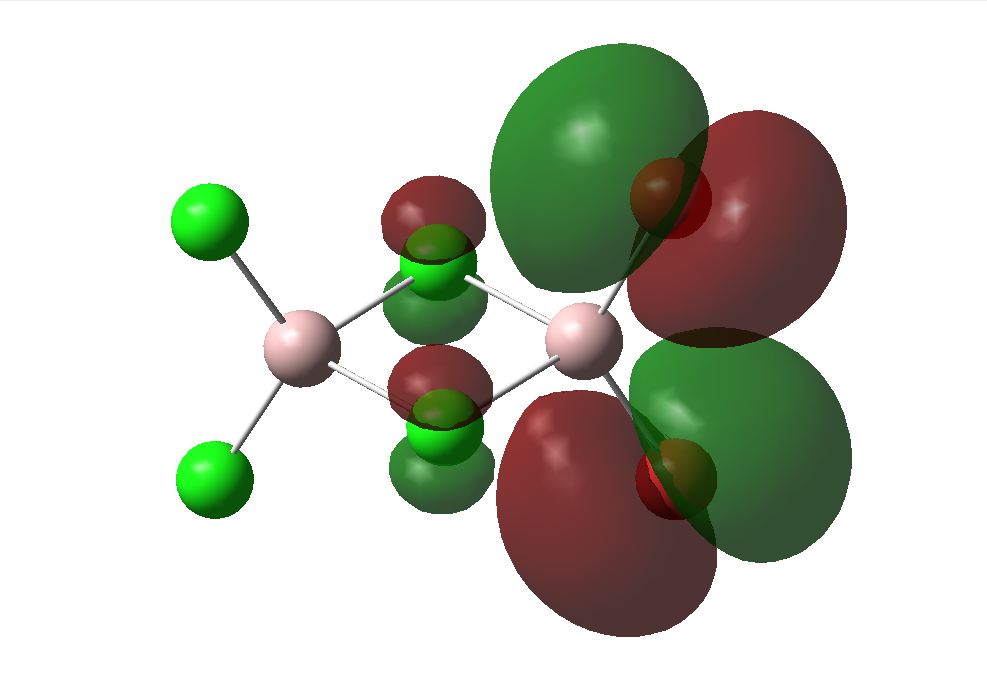
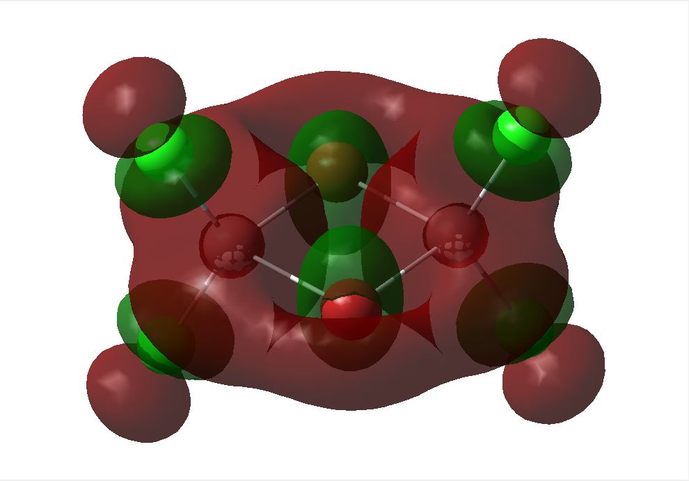
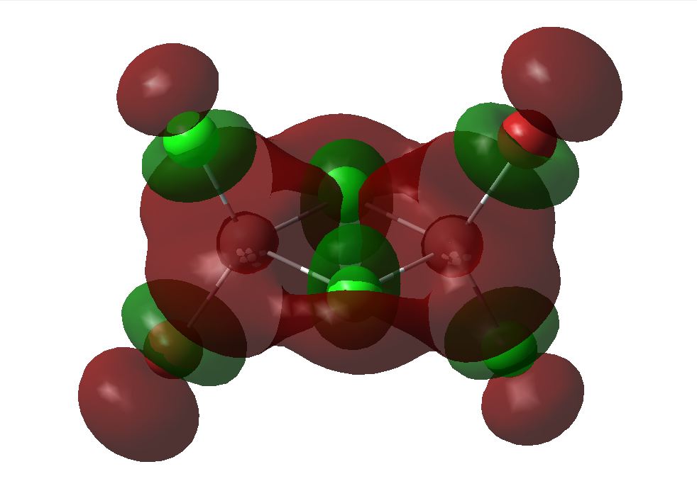
Molecular Orbital Analysis
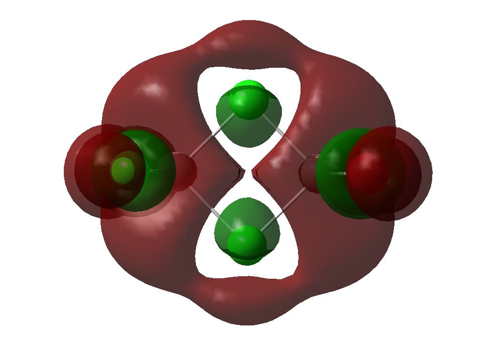
The optimised geometry from the LANL2DZ basis set was used to calculate the MOs of the three structures under investigation. The HOMO and LUMOs of the stuctures are shown below. This basis set determined the cis to be the most thermodynamically favoured. This can be supported by the LUMO of the cis shown below. Its can be seen that the overlap between the cis and trans LUMO between the central bridging chlorines and the Aluminiums are better than that in teh bridging molecule, since there is a mismatch of size of teh orbitals in teh bridging structure. The energies of the MOs are associated with the relative amounts of favourable and unfavourable interaction between orbitals. This calculation does not take the diffusion or polarisability of orbitals into account however, so it is likely that a different outcome will be seen when using the more complex basis set.
| Bridging | Cis | Trans | |
| HOMO |  |
 |
|
| LUMO |  |
 |
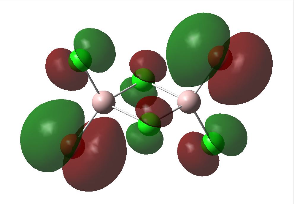
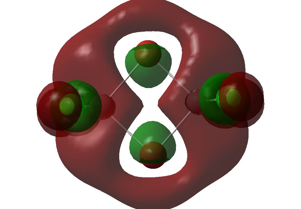
The 6-31G+d,p optimised geometry was also used to determine the MOs of the three structures to see if there was any difference compared to the simpler basis set. The energy calculations were sent to SCAN [35][36][37]. It was interesting to see that the HOMOs had the same MOs however the LUMOs were different. The MOs predicted using the 6-31G+d,p basis set show better interaction between the orbitals. The orbitals are more diffuse and less structured than that for the simpler basis set. These are more accurate predictions of the MOs that would be expected from an MO diagram since the calculation takes into account the diffusion and polarisation as well as the p and d orbital contribution. From the 6-31G+d,p basis set MOs The Birds eye view images of the LUMO show that the bridging LUMO has the most favourable interaction and would therefore be the most stable, it is also lower in energy (-0.06656 Ha) compared to the cis (-0.06593 Ha), and both are lower than the trans (-0.06498Ha). This fits with the conclusion from the optimised geometry. Since the LUMOs have negative energies, it is possible to add a pair of electrons without destabilising the energy of the molecule, therefore it is possible for the bridging, cis and trans structures of [Al2Cl4Br2]2- to exist.
6-31G+d,p Basis Set MOs| Bridging | Cis | Trans | |
| HOMO |  |
 |
|
| LUMO |  |
 |
|
| MO Energies |  |
 |
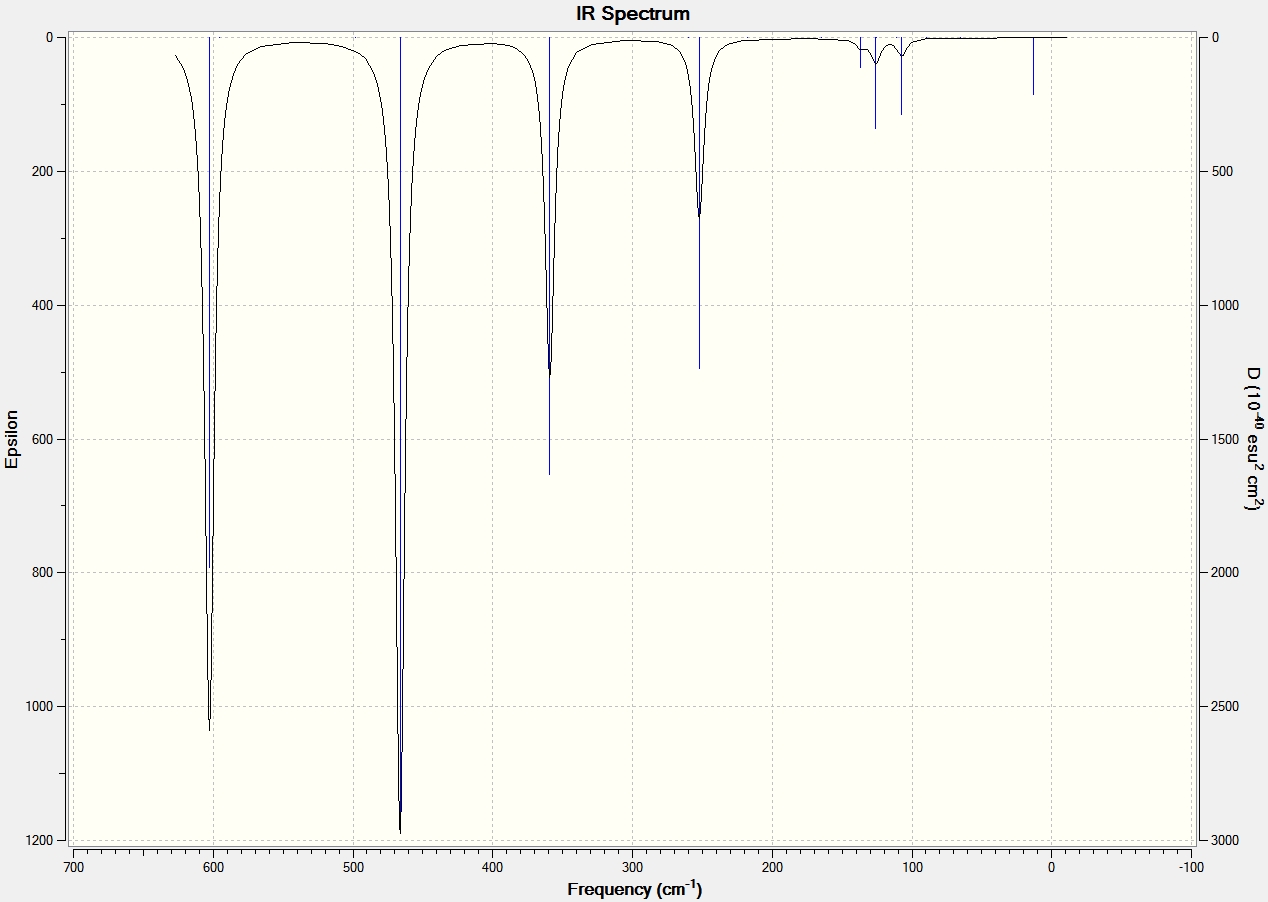
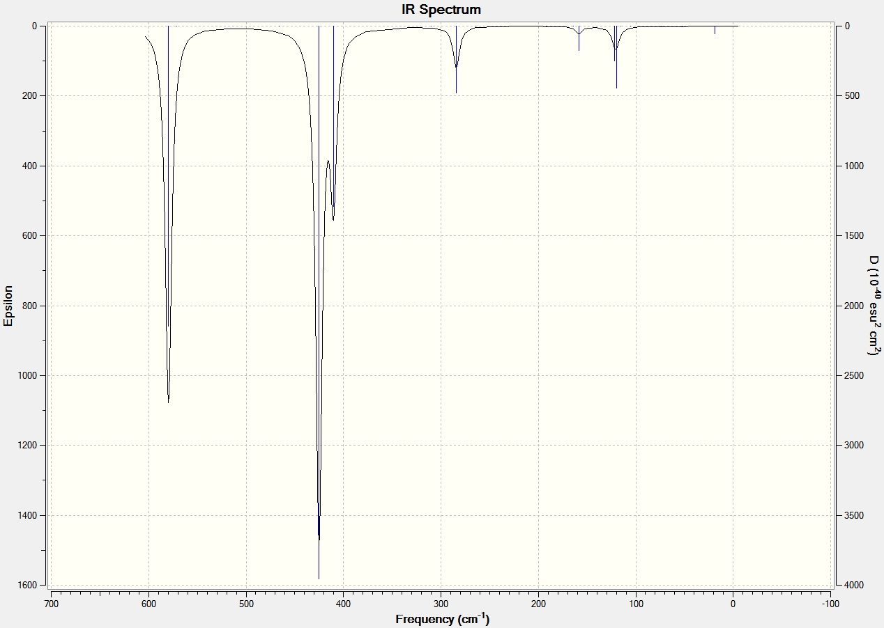
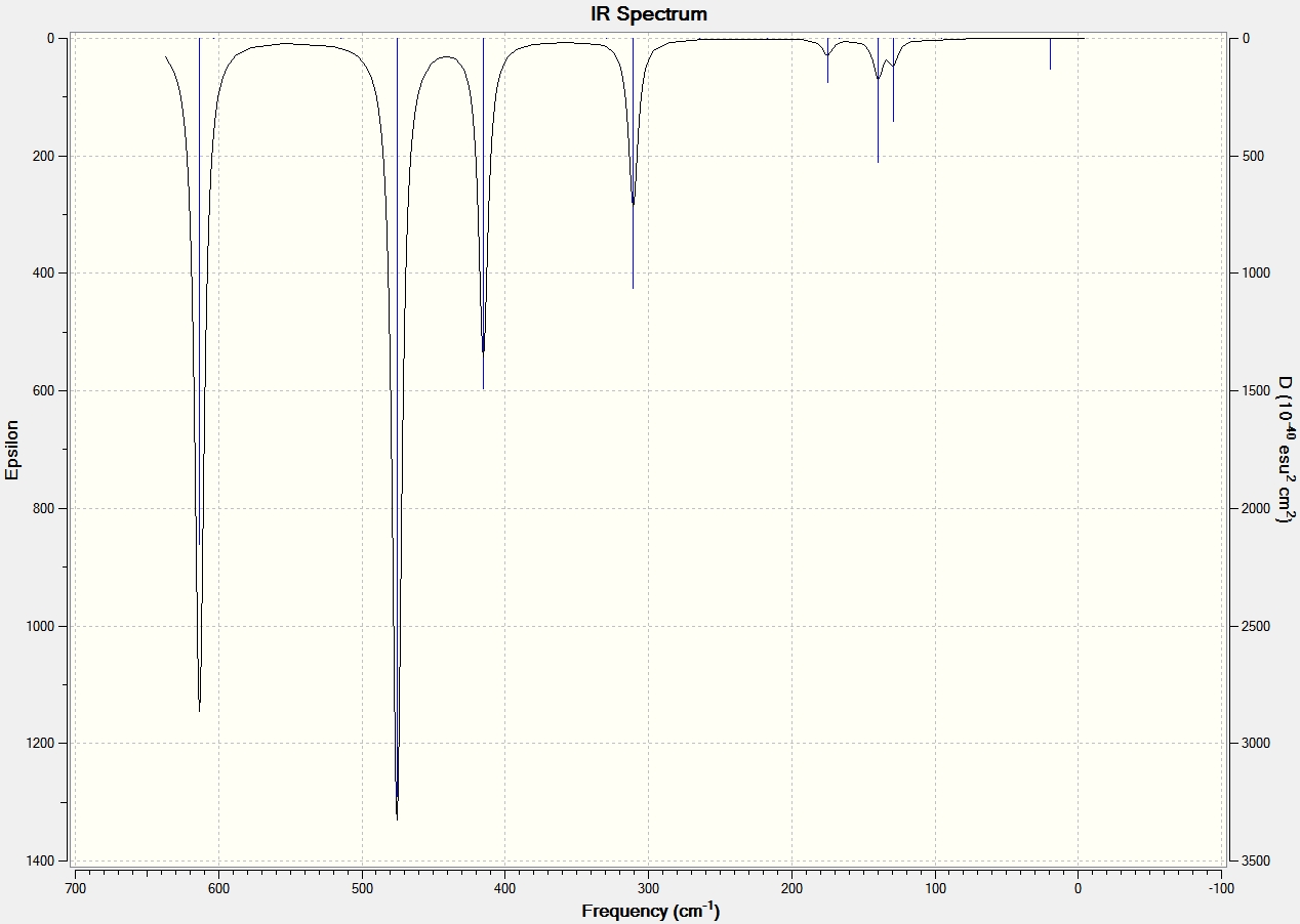
Frequency Analysis
The Frequency was calculated by using the B3YLP method and the 6-31G+d,p basis set as the above analysis concluded that this basis set was the most accurate in predicting properties of the structures. The calculation was sent to SCAN [38][39][40][41]. The frequency summaries are shown below:
6-31G+d,p Basis Set Frequency Summary |
 |
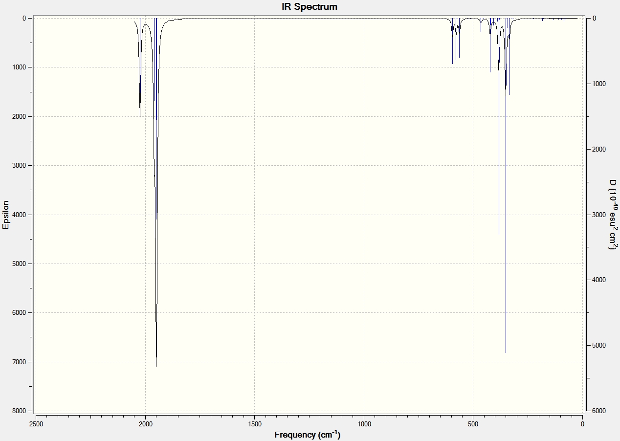
The vibrational modes were viewed on GaussView and the spectral data is shown below along with the spectrums of each structure. The data clearly shows that the cis structure has the most stretching frequency. This is because the trans and bridging structure have a more symetrical structure when in comes to vibrational modes and so alot of the stretching of the bonds essentially cancel out and produce no overall dipole. Therefore they are not seen in any stretching frequencies. This is supported by the frequency summary above which shows that the bridging and trans structures have dipole moments close to 0 Debye, whereas the cis structure has a dipole moment of 0.9075 Debye. All the structures exhibit three main vibrational modes that produce a dipole moment and therefore show on the IR spectrum. The first is the forward and back rocking of the Aluminium atoms whilst the halides remain static. This vibrational mode is seen at 359 cm-1, 412 cm-1 and 410cm-1 for the bridging, cis and trans structures respectively. The Bridging stretching frequency is lower since the bridging Br have a longer and therefore weaker bond to the Al atoms. The second vibrational mode seen is the aluminium atoms moving from left to right asymmetrically whilst the halides remain still. The relative frequencies for the bridging and trans structures are 466cm-1 and 425cm-1 respectively. The cis exhibits two stretching frequencies for this vibrational mode, at 417cm-1 and 502cm-1, where it is attached to the Br terminal and Cl terminal respectively. The Br terminal has a lower stretching frequency since the Br-Al bond is weaker than the Cl-Al bond. The third and final vibrational mode is the aluminium atoms moving up and down symmetrically whilst the halides remain static. This vibrational mode is seen at 602 cm-1 and 579 cm-1 for the bridging and trans structures respectively. Again the cis structure exhibits two stretching frequencies for this vibrational mode, at 529 cm-1 and 604 cm-1, where it is attached to the Br terminal and Cl terminal respectively. The same reason as before accounts for the lower Br-Al stretching frequency. No negative frequencies were found for any of the structures suggesting that a global minimum had been found.
IR Data for Aluminium Dimers |
 |
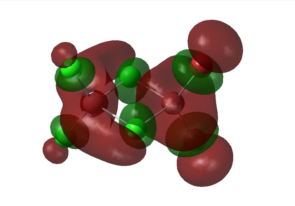
Charge Distribution Analysis
The charge distributions were found from the frequency calculations that were sent to SCAN [42][43][44][45]. The charges for each atom are shown in the images below. As expected, it can be seen that the chlorine atoms are more negative than the bromine and this is explained by the relative electronegativities of the chlorine and bromine. Chlorine is more electronegative than bromine so it holds onto electron density more, therefore it has a greater negative charge. When looking at the Aluminium atoms it can be seen that in the bridging and trans structures, the aluminium has the same positive charge. However in the cis structure the aluminium atoms has asymmetric charge distribution. The aluminium with two terminal chlorine atoms is more positively charged than the aluminium with the two terminal bromine atoms. This is because the chlorine is more electronegative, so the aluminium attached to two terminal chlorines is more deshielded. It is also noticeable that the bridging halides are less negatively charged than if they were placed in the terminal position. This demonstrates that the 3c-2e bond is electron deficient.
 |
 |
Gallium Structure
Gallium was substituted for aluminium to make a gallium dimer - Ga2Cl6. The geometry was optimised using the B3YLP method and 6-3G1+d,p basis set and sent to SCAN [46]. The frequency was also calculated using teh sam settings via SCAN[47]. The aluminium dimer investigation was taken into consideration when chosing the method and basis set for gallium in order to produce the most accurate results. This structure was investigated to show how a heavier atom affects the energy, vibrational modes and charge distribution. The optimisation and frequency summaries for gallium and aluminium dimers are shown below:
 |
 |
|
 |
The RMS gradient norm is very close to zero suggesting that a miniumum energy configuration was found and that the calculations converged. The dipole moment is as expected and is zero since the molecule is very symmetrical. The bond measurements were found using GaussView and are tabulated below:
| Bond Measuremenents of Ga2Cl6 | Ga2Cl6 |
|---|---|
| Bridging Ga-Cl-Ga angle (degrees) | 90.0 |
| Bridging Cl-Ga-Cl angle (degrees) | 90.0 |
| Terminal Cl-Ga-Cl angle (degrees) | 122.0 |
| Bridging Ga-Cl bond distance (angstroms) | 2.48 |
| Terminal Ga-Cl bond distance (angstroms) | 2.24 |
This can be compared to the data collected for the Al2Cl6 structure (shown in a table above). The values for the bond angles are very similar however the bond distances are slightly different to that of the aluminium strutcure. They are generally longer than in the aluminium structure which can be explained by the fact that Gallium is a larger atom and therefore the bond length is longer. Aluminium is also close to chlorine in the periodic table therefore has better overlap of orbitals so would expect to have stronger and therefore shorter bonds. There is not a vast amount of difference however since the d orbitals have been considered in the calculation which would improve the interaction for the Gallium and hence shorten the Ga-Cl bond, essentially conteracting the size of Gallium.
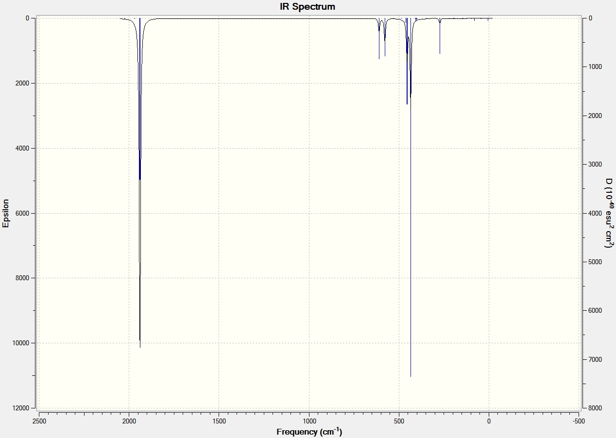
IR Data for Al2Cl6 and Ga2Cl6 |
 |
From the IR data it can be seen that both structures have 8 visibly stretching frequencies that show on the IR spectrum. This is as expected since the molecules are very similar in structure. No more than 8 are visible on the spectrum since both structures are highly symmetric with a dipole moment close to 0 Debye. Therefore many of the vibrations and stretches of teh bonds essentially cancel out to give no overall dipole moment. The Gallium frequencies are generally much lower than the Aluminium frequencies and this is because the reduced mass of the two gallium atoms is much greater than that of the aluminium.
The charge distribution was found by sending an energy calculation to SCAN [48][49] using the same method and basis set as the optimisation calculation. The comparison of charge distributions between Al2Cl6 and Ga2Cl6 are shown below:
Charge Distribution for Al2Cl6 and Ga2Cl6 |
 |
It can be seen that the chlorines are less negative in the Gallium structure compared to the Aluminium structure. This suggests that the dipole moment for each bond is less extreme than in the Aluminium structure. Both molecules are symmetric therefore it can be seen that the charge distribution is also symmetric.
Conclusion
The mini project has demonstrated the importance of parameters in computational chemistry. It is essential to consider the basis sets and pseudo potentials used in a calculation as using different ones for more complex molecules may give varying conclusions as seen above. It was also able to show that more complex molecules and molecules with heavier atoms are able to be analysed computationally. For example it showed that the unusual structure of Diborane is also found in molecules with heavier elements and halogens.
The mini project was able to distinguish the three aluminium isomers through IR analysis, molecular orbital analysis and charge distribution analysis.
It was also able to show that heavier elements such as Gallium can also form a bridging structure.
With more time it would be interesting to investigate more pseudo potentials and their affects on predicting molecules properties and structures. Molecules with even heavier elements could also be investigated.
References
- ↑ 3rd Year Computational Chemistry Online Lab Manual, Module 2, 2011
- ↑ J. Nørskov et al., Chemistry World, 05 June 2008
- ↑ M. S. Schuurman et al., J. Comp. Chem., 26(11), 2005, pp 1106
- ↑ W.H.Brown et al., Organic Chemistry, Sixth Edition, 2010, pp 237
- ↑ B. Khater et al., J. Chem. Phys., 129(22), 2008
- ↑ http://hdl.handle.net/10042/to-12044
- ↑ P. Hunt, 2nd Year Inorganic Chemistry Course - Molecular Orbitals In Inorganic Chemistry, 2010
- ↑ J. Mullay, J. Am. Chem. Soc., 106, 1984, pp 5842 - 5847
- ↑ M. Anatosov et al., J. Phys. Chem., 105, 2001, pp 5450 - 5467
- ↑ J. Blixt et al., J. Am. Chem. Soc., 117, 1995, pp 5089 - 5104
- ↑ J. E. D. Davies et al., J. Chem. Soc. (A), 1968, pp 2050 - 2054
- ↑ http://hdl.handle.net/10042/to-12048
- ↑ http://hdl.handle.net/10042/to-12047
- ↑ http://hdl.handle.net/10042/to-12043
- ↑ http://hdl.handle.net/10042/to-12042
- ↑ http://hdl.handle.net/10042/to-12039
- ↑ http://hdl.handle.net/10042/to-12038
- ↑ A. D. Allen et al., Can. J. Chem., 46, 1968 pp 1649 – 1653
- ↑ N. M. Xiang, et. al, Universiti Teknologi Malaysia, Identification of Stereochemical Isomers by Infrared Spectroscopy, 2010, pp 15
- ↑ F. A. Cotton, Inorg. Chem., 21, 1982, pp 294 - 299
- ↑ D. W. Bennett, J. Chem. Cryst., 34(6), 2004, pp 353 - 359
- ↑ http://hdl.handle.net/10042/to-12037
- ↑ http://hdl.handle.net/10042/to-12036
- ↑ http://hdl.handle.net/10042/to-12032
- ↑ http://hdl.handle.net/10042/to-12033
- ↑ P. Hunt, 2nd Year Inorganic Chemistry Course - Molecular Orbitals In Inorganic Chemistry, 2010
- ↑ http://hdl.handle.net/10042/to-12031
- ↑ http://hdl.handle.net/10042/to-12030
- ↑ http://hdl.handle.net/10042/to-12027
- ↑ http://hdl.handle.net/10042/to-12026
- ↑ http://hdl.handle.net/10042/to-12023
- ↑ http://hdl.handle.net/10042/to-12022
- ↑ http://hdl.handle.net/10042/to-12021
- ↑ K. Wade, J. Chem. Educ., 49(7), 1972, pp 502
- ↑ http://hdl.handle.net/10042/to-12016
- ↑ http://hdl.handle.net/10042/to-12015
- ↑ http://hdl.handle.net/10042/to-12014
- ↑ http://hdl.handle.net/10042/to-12020
- ↑ http://hdl.handle.net/10042/to-12019
- ↑ http://hdl.handle.net/10042/to-12018
- ↑ http://hdl.handle.net/10042/to-12017
- ↑ http://hdl.handle.net/10042/to-12020
- ↑ http://hdl.handle.net/10042/to-12019
- ↑ http://hdl.handle.net/10042/to-12018
- ↑ http://hdl.handle.net/10042/to-12017
- ↑ http://hdl.handle.net/10042/to-12013
- ↑ http://hdl.handle.net/10042/to-12012
- ↑ http://hdl.handle.net/10042/to-12011
- ↑ http://hdl.handle.net/10042/to-12010