Rep:Mod:fyl10y3
Third Year Computational Chemistry Laboratory: Module 2
LOO, Fai-Yang Ferdinand (00641123)
Week 1: Basic Calculations
Optimisation of BH3, TlBr3 and BBr3
Optimisation of BH3 using B3LYP with the 3-21G Basis Set
Creating and Optimising the Molecule
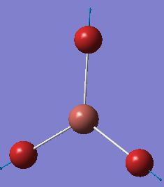
A molecule of BH3 was set up in GaussView and the three B-H bond distances were set to be 1.5 angstroms. The molecule was then optimised using Gaussian:
- method: B3LYP
- basis set: 3-21G
- type of calculation: OPT
This method is of low accuracy but takes only a short time to complete. The .log file of the optimised molecule can be found here.
Analysing the Optimised Molecule
From the optimised BH3 molecule the B-H bond distance and H-B-H bond angles were calculated:
- B-H distance: 1.19 angstroms
- H-B-H angle: 120.0 degrees
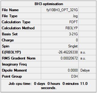
Gaussian calculation summary for the Optimisation of BH3 molecule using the B3LYP method and 3-21G basis set:
Check for proper optimisation (i.e. Gradient should be <0.001):
- A gradient of 0.00020672 a.u. implies optimisation was properly done.
Extraction from Gaussian file:
         Item               Value     Threshold  Converged?
 Maximum Force            0.000413     0.000450     YES
 RMS     Force            0.000271     0.000300     YES
 Maximum Displacement     0.001610     0.001800     YES
 RMS     Displacement     0.001054     0.001200     YES
 Predicted change in Energy=-1.071764D-06
 Optimization completed.
    -- Stationary point found.
                           ----------------------------
                           !   Optimized Parameters   !
                           ! (Angstroms and Degrees)  !
 --------------------------                            --------------------------
 ! Name  Definition              Value          Derivative Info.                !
 --------------------------------------------------------------------------------
 ! R1    R(1,2)                  1.1935         -DE/DX =    0.0004              !
 ! R2    R(1,3)                  1.1935         -DE/DX =    0.0004              !
 ! R3    R(1,4)                  1.1935         -DE/DX =    0.0004              !
 ! A1    A(2,1,3)              120.0            -DE/DX =    0.0                 !
 ! A2    A(2,1,4)              120.0            -DE/DX =    0.0                 !
 ! A3    A(3,1,4)              120.0            -DE/DX =    0.0                 !
 ! D1    D(2,1,4,3)            180.0            -DE/DX =    0.0                 !
 --------------------------------------------------------------------------------
 GradGradGradGradGradGradGradGradGradGradGradGradGradGradGradGradGradGrad
Optimisation of BH3 using B3LYP with the 6-31G(d,p) Basis Set
Creating and Optimising the Molecule
A molecule of BH3 was set up in GaussView and the three B-H bond distances were set to be 1.5 angstroms. The molecule was then optimised using Gaussian:
- method: B3LYP
- basis set: 6-31G (d,p)
- type of calculation: OPT
This is a higher level basis set following the last one. The .log file of the optimised molecule can be found here.
Analysing the Results from the Second Optimisation
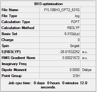
Gaussian calculation summary for the Optimisation of BH3 molecule using the B3LYP method and the 6-31G(d,p) basis set:
A small enough gradient of 0.00021692 a.u. has confirmed a successful optimisation.
The item table is also included for confirmation of a successful optimisation:
Item               Value     Threshold  Converged?
 Maximum Force            0.000433     0.000450     YES
 RMS     Force            0.000284     0.000300     YES
 Maximum Displacement     0.001702     0.001800     YES
 RMS     Displacement     0.001114     0.001200     YES
 Predicted change in Energy=-1.189019D-06
 Optimization completed.
    -- Stationary point found.
                           ----------------------------
                           !   Optimized Parameters   !
                           ! (Angstroms and Degrees)  !
 --------------------------                            --------------------------
 ! Name  Definition              Value          Derivative Info.                !
 --------------------------------------------------------------------------------
 ! R1    R(1,2)                  1.1914         -DE/DX =    0.0004              !
 ! R2    R(1,3)                  1.1914         -DE/DX =    0.0004              !
 ! R3    R(1,4)                  1.1914         -DE/DX =    0.0004              !
 ! A1    A(2,1,3)              120.0            -DE/DX =    0.0                 !
 ! A2    A(2,1,4)              120.0            -DE/DX =    0.0                 !
 ! A3    A(3,1,4)              120.0            -DE/DX =    0.0                 !
 ! D1    D(2,1,4,3)            180.0            -DE/DX =    0.0                 !
 --------------------------------------------------------------------------------
 GradGradGradGradGradGradGradGradGradGradGradGradGradGradGradGradGradGrad
Bond lengths and bong angles:
- Optimised B-H length: 1.19 angstroms
- Optimised H-B-H angle: 120.0 degrees
Comparison of the Optimisation Results of BH3 using B3LYP with the 3-21G and 6-31G(d,p) Basis Sets
Total energies: Method for both optimisations: B3LYP
- Using the 3-21G basis set: -26.46226338 a.u.
- Using the 6-31G(d,p) basis set: -26.61532252 a.u.
The result obtained using the 6-31G(d,p) basis set is more negative by 0.15305914 a.u., however, they are not directly comparable due to having different basis-sets. Only optimisations using exactly the same method and basis set can be directly compared.
Optimisation of the TlBr3 Molecule
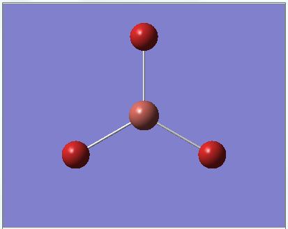
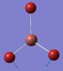
Molecule was setup in GaussView and optimised using B3LYP with the LanL2DZ basis set, with the symmetry restricted to be D3h and the tolerance threshold set to "very tight(0.0001)". The .gjf file was modified and submitted to HPC, which yielded a .log file and was examined in GaussView to check if the optimisation was done properly:
The file was then published to the chemical database D-Space and can be found here: [1]
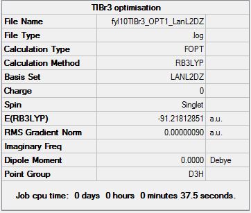
The summary file of the optimised molecule is also shown below:
A very small gradient of 0.00000090 a.u. and all converging values (to be found below) is evident of a successful optimisation.
The Item table is also included for proof of proper optimisation:
Item               Value     Threshold  Converged?
 Maximum Force            0.000002     0.000450     YES
 RMS     Force            0.000001     0.000300     YES
 Maximum Displacement     0.000022     0.001800     YES
 RMS     Displacement     0.000014     0.001200     YES
 Predicted change in Energy=-6.084046D-11
 Optimization completed.
    -- Stationary point found.
                           ----------------------------
                           !   Optimized Parameters   !
                           ! (Angstroms and Degrees)  !
 --------------------------                            --------------------------
 ! Name  Definition              Value          Derivative Info.                !
 --------------------------------------------------------------------------------
 ! R1    R(1,2)                  2.651          -DE/DX =    0.0                 !
 ! R2    R(1,3)                  2.651          -DE/DX =    0.0                 !
 ! R3    R(1,4)                  2.651          -DE/DX =    0.0                 !
 ! A1    A(2,1,3)              120.0            -DE/DX =    0.0                 !
 ! A2    A(2,1,4)              120.0            -DE/DX =    0.0                 !
 ! A3    A(3,1,4)              120.0            -DE/DX =    0.0                 !
 ! D1    D(2,1,4,3)            180.0            -DE/DX =    0.0                 !
 --------------------------------------------------------------------------------
 GradGradGradGradGradGradGradGradGradGradGradGradGradGradGradGradGradGrad
- Optimised Tl-Br bond length: 2.65 angstroms
- Optimised Br-Tl-Br bond angle: 120.0 degrees
The obtained Tl-Br bond length of 2.65 angstroms is close to the 2.512 angstroms found in literature data [1], only with a small percentage difference of 5.5%. The optimisation was properly done and analysis was proceeded.
Optimisation of the BBr3 Molecule
A molecule of BBr3 was created on GaussView based on the optimised BH3 molecule.The optimised file was uploaded onto D-Space and can be found here [2].
The same method was used but with different basis sets, a full basis set of 6-31G(d,p) was used for B and a pseudo-potential of LanL2DZ on the heavier Br atoms.
Summary of optimisation:
- Method: B3LYP
- Basis set for B: 6-31G(d,p)
- Basis set for Br: LanL2DZ
The HPC optimised molecule was examined in GaussView and seemed reasonable, with all expected bonds present and a reasonable geometry. A gradient of 0.00000382 a.u. which is small and all converging values proved that the optimisation was successful.
The summary of the optimised molecule was also recorded as follows:
The optimisation was also complete, showed by the convergence of the optimisation steps. The Items content also included:
Item               Value     Threshold  Converged?
 Maximum Force            0.000008     0.000450     YES
 RMS     Force            0.000005     0.000300     YES
 Maximum Displacement     0.000036     0.001800     YES
 RMS     Displacement     0.000023     0.001200     YES
 Predicted change in Energy=-4.026779D-10
 Optimization completed.
    -- Stationary point found.
                           ----------------------------
                           !   Optimized Parameters   !
                           ! (Angstroms and Degrees)  !
 --------------------------                            --------------------------
 ! Name  Definition              Value          Derivative Info.                !
 --------------------------------------------------------------------------------
 ! R1    R(1,2)                  1.934          -DE/DX =    0.0                 !
 ! R2    R(1,3)                  1.934          -DE/DX =    0.0                 !
 ! R3    R(1,4)                  1.934          -DE/DX =    0.0                 !
 ! A1    A(2,1,3)              120.0            -DE/DX =    0.0                 !
 ! A2    A(2,1,4)              120.0            -DE/DX =    0.0                 !
 ! A3    A(3,1,4)              120.0            -DE/DX =    0.0                 !
 ! D1    D(2,1,4,3)            180.0            -DE/DX =    0.0                 !
 --------------------------------------------------------------------------------
 GradGradGradGradGradGradGradGradGradGradGradGradGradGradGradGradGradGrad
Calculation results are shown:
- Optimised B-Br bond distance: 1.93 angstroms
- Optimised Br-B-Br bond angle: 120.0 degrees
Summary and Comparison of BH3, BBr3, TlBr3 Bond Distances
| BH3 | BBr3 | TlBr3 |
|---|---|---|
| 1.19 angstroms | 1.93 angstroms | 2.65 angstroms |
1. Comparing the BH3, BBr3 and TlBr3 calculation results
Different ligands have different number of electrons, different number of orbitals and hence a different atomic size. Outer orbitals are larger and more diffuse in electron density, leading to poorer overlap. The symmetry of overlapping orbitals also contribute to the degree of overlap, which a larger overlap leads to closer energy levels and therefore a greater energy shift of the resulting MO's. These factors contribute to the degree of overlap of the centre and the ligand, for a smaller size mismatch, the overlap will be stronger and hence a stronger and shorter bond, vice versa. So for a different ligand it has a different size and hence the overlap and bond energy will be affected. The H and Br ligands are both X ligands, meaning they are ligands naturally carrying one negative charge and donates one electron to the centre per H or Br atom upon coordination to the central atom. However, the Br atom is much larger, having many more electron shells and more diffuse orbitals, therefore the overlap with the B centre is poor, due to having a small overlap integral compared to that between H and B. H on the other hand, is small in size and concentrated in charge, having a smaller orbital size mismatch with the B centre and the bond between is much stronger, leading to a significantly shorter bond distance of 1.19143 angstroms, whereas the B-Br bond distance is almost two times of that.
The central element (centre) is also important in contributing to the overall bond strengths and lengths. Comparing BBr3 and TlBr3, TlBr3 has a much longer bond distance. This can be explained in a similar manner, in the sense that, the Tl atom is larger and more diffuse than the B centre, leading to a poorer overlap between the Tl and Br atoms and hence a weaker, longer bond. B and Tl are both Group 13 elements and are both electron deficient in nature, but Tl being much lower in the periodic table has a larger number of orbitals and the bonding orbital is very diffuse with only a low electron density leading to poor overlaps with the Br ligand.
All three molecules, however, have the same bond angles of 120 degrees. This is because the bonds are equivalent in all three cases, and the centres possess no electron lone pairs, so all three molecules have trigonal planar structures and have optimised bond angles of 120.0 degrees in each case, corresponding to the D3h symmetry.
2. Discussion of bonding in Gaussview
In some structure GaussView does not show the bonds that we expect from the structure, since GaussView identifies bonds based on a distance criteria, i.e. the bonds that were not drawn have exceeded a pre-defined distance. The bond not being shown does not mean that it does not exist, it is just that the program does not recognise it as a bond which has to satisfy the preset distance threshold and is not presented in the structure drawn. A bond can be of several natures, depending on the electronegativity difference between the bonding atoms. In this analysis, all three molecules BH3, BBr3 and TlBr3 have a small electronegativity difference and are majorly covalent in nature. The bonds here are defined as a sharing of electron density between the atoms, via overlapping of the atomic orbitals of the bonding atoms. In some cases the bonds may be long,exceeding the pre-defined value set in GaussView and thus is not presented, however, this just means the bond might be weak corresponding to a long bond, but does not mean that the bond does not exist.
Frequency and Energetic Analysis for BH3, TlBr3 and BBr3
Frequency Analysis for BH3
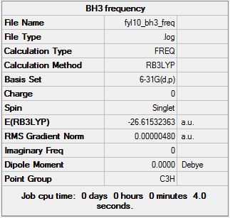
The optimised model was processed in a frequency analysis and the processed file can be found here.
Comparing to the pre-frequency-analysed file, it has the same energy of -26.61532252 a.u..
The summary of the frequency analysis is posted below:
The Item section of the file is also recorded as follows:
Low frequencies ---   -3.6018   -1.1356   -0.0054    1.3735    9.7036    9.7698
 Low frequencies --- 1162.9825 1213.1733 1213.1760
 Harmonic frequencies (cm**-1), IR intensities (KM/Mole), Raman scattering
 activities (A**4/AMU), depolarization ratios for plane and unpolarized
 incident light, reduced masses (AMU), force constants (mDyne/A),
 and normal coordinates:
                     1                      2                      3
                    A"                     E'                     E'
 Frequencies --  1162.9825              1213.1733              1213.1760
 Red. masses --     1.2531                 1.1072                 1.1072
 Frc consts  --     0.9986                 0.9601                 0.9601
 IR Inten    --    92.5497                14.0545                14.0581
  Atom  AN      X      Y      Z        X      Y      Z        X      Y      Z
     1   5     0.00   0.00   0.16     0.00   0.10   0.00    -0.10   0.00   0.00
     2   1     0.00   0.00  -0.57     0.00   0.08   0.00     0.81   0.00   0.00
     3   1     0.00   0.00  -0.57    -0.39  -0.59   0.00     0.14   0.39   0.00
     4   1     0.00   0.00  -0.57     0.39  -0.59   0.00     0.14  -0.39   0.00
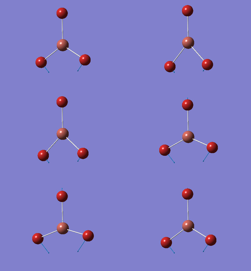
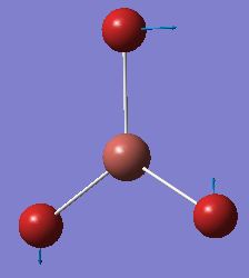
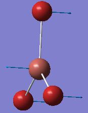
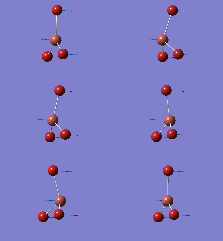
The "Low frequencies" values reflects the degree of freedom of the molecule, representing the "-6" part of the 3N-6 value of the optimised molecule. It should lie within the range of +-15cm-1. In this case, it can be seen in the pasted Item section that the largest value is +9.7698cm-1, which is smaller than 15 and is acceptable. The first vibration has a frequency of 1163cm-1, which is about two order of magnitude larger than the largest "low frequency" calculated. However, upon checking the "real frequencies", it has the wrong symmetry label of A", as opposed to the expected A2" which corresponds to a D3h symmetry of the molecule. Therefore the optimisation and frequency calculation was re-done and shown in the part below.
Repeating the Optimisation and Frequency Analysis of BH3
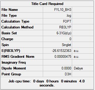
The BH3 molecule was set up and optimised using the B3LYP method with the basis sets 3-21G and 6-31G(d,p). The .log file of the re-optimised BH3 molecule can be found here.
It has an energy of -26.61532363 a.u. and the summary of the optimised molecule is shown here:
The Item section is shown here:
Item               Value     Threshold  Converged?
 Maximum Force            0.000009     0.000450     YES
 RMS     Force            0.000006     0.000300     YES
 Maximum Displacement     0.000038     0.001800     YES
 RMS     Displacement     0.000025     0.001200     YES
 Predicted change in Energy=-5.343321D-10
 Optimization completed.
    -- Stationary point found.
                           ----------------------------
                           !   Optimized Parameters   !
                           ! (Angstroms and Degrees)  !
 --------------------------                            --------------------------
 ! Name  Definition              Value          Derivative Info.                !
 --------------------------------------------------------------------------------
 ! R1    R(1,2)                  1.1923         -DE/DX =    0.0                 !
 ! R2    R(1,3)                  1.1923         -DE/DX =    0.0                 !
 ! R3    R(1,4)                  1.1923         -DE/DX =    0.0                 !
 ! A1    A(2,1,3)              120.0            -DE/DX =    0.0                 !
 ! A2    A(2,1,4)              120.0            -DE/DX =    0.0                 !
 ! A3    A(3,1,4)              120.0            -DE/DX =    0.0                 !
 ! D1    D(2,1,4,3)            180.0            -DE/DX =    0.0                 !
 --------------------------------------------------------------------------------
 GradGradGradGradGradGradGradGradGradGradGradGradGradGradGradGradGradGrad
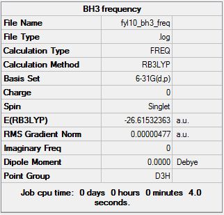
The optimised molecule has its symmetry label restricted to the D3h symmetry with a very tight tolerance set, and the calculation was repeated. The new log file can be found here.
The summary is posted below:
The Item section is shown below as well:
Low frequencies ---   -3.5991   -1.1355   -0.0055    1.3745    9.7046    9.7707
 Low frequencies --- 1162.9825 1213.1733 1213.1760
It can be seen that the "Low frequencies" remain similar, and the symmetry label of the first "Real frequency" is correct now. The energy is now -26.61532363 a.u. which is identical to the -26.61532363 a.u. obtained before doing the frequency analysis. The frequency calculation is correctly repeated and moved on to the next step.
Infrared Spectrum Prediction from Frequency Analysis of BH3
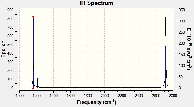
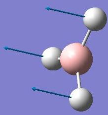
The IR spectrum is predicted using Gaussian form the BH3 frequency analysis file. The spectrum obtained is shown below:
The absorptions are also tabulated:
The table shows 6 absorptions, while only 3 major peaks are observed in the spectrum shown. This is because modes #2 and #3 both have 1213cm-1 absorptions and #5 and #6 have 2715cm-1. The two sets stick really close and are very hard to differentiate. The remaining #4 at 2582cm-1 has an absorption too low to be observed on the spectrum. The sets of absorptions have nearly identical absorption frequencies because the absorptions have nearly the same energy capacity and hence have very close frequencies absorbed on the IR spectrum.
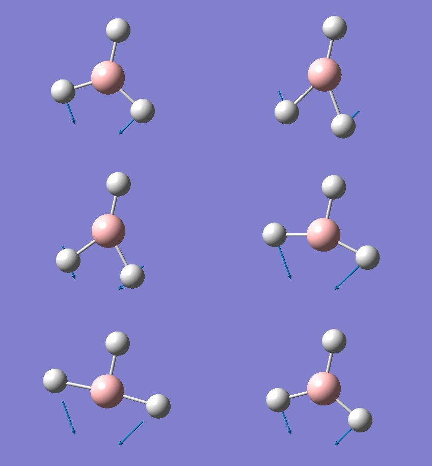
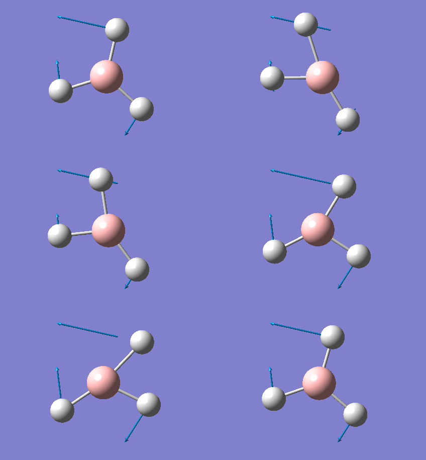
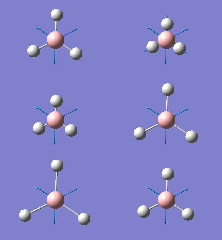
The absorptions, intensities, form of vibration and its corresponding symmetry label are summarised in the table below:
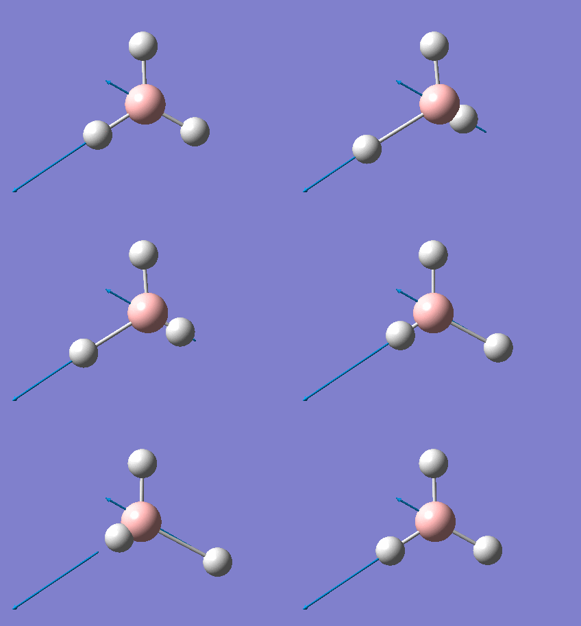
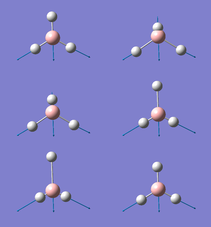
Frequency Analysis of the Optimised TlBr3 Molecule
The completed analysis of the molecule is uploaded to D-Space and the link can be found here:
The "Low Frequency" Information is also shown below:
Low frequencies ---   -0.0008   -0.0004   -0.0003   18.6824   19.5013   19.5013
 Low frequencies ---   49.9765   49.9768   57.4605
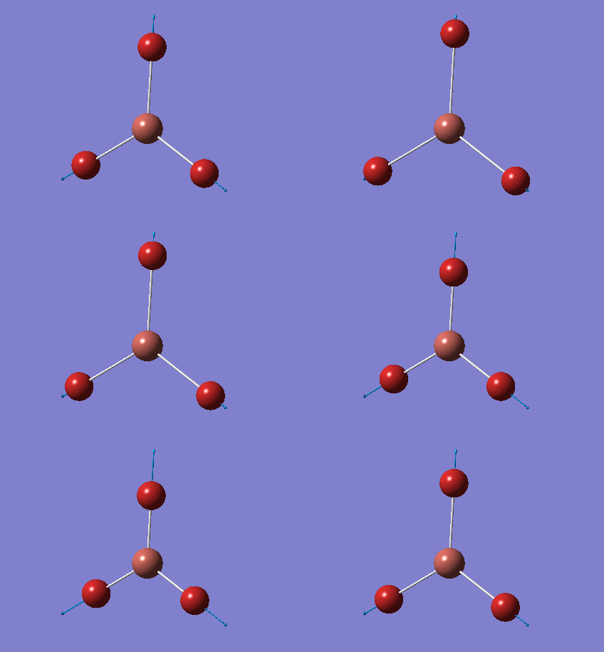
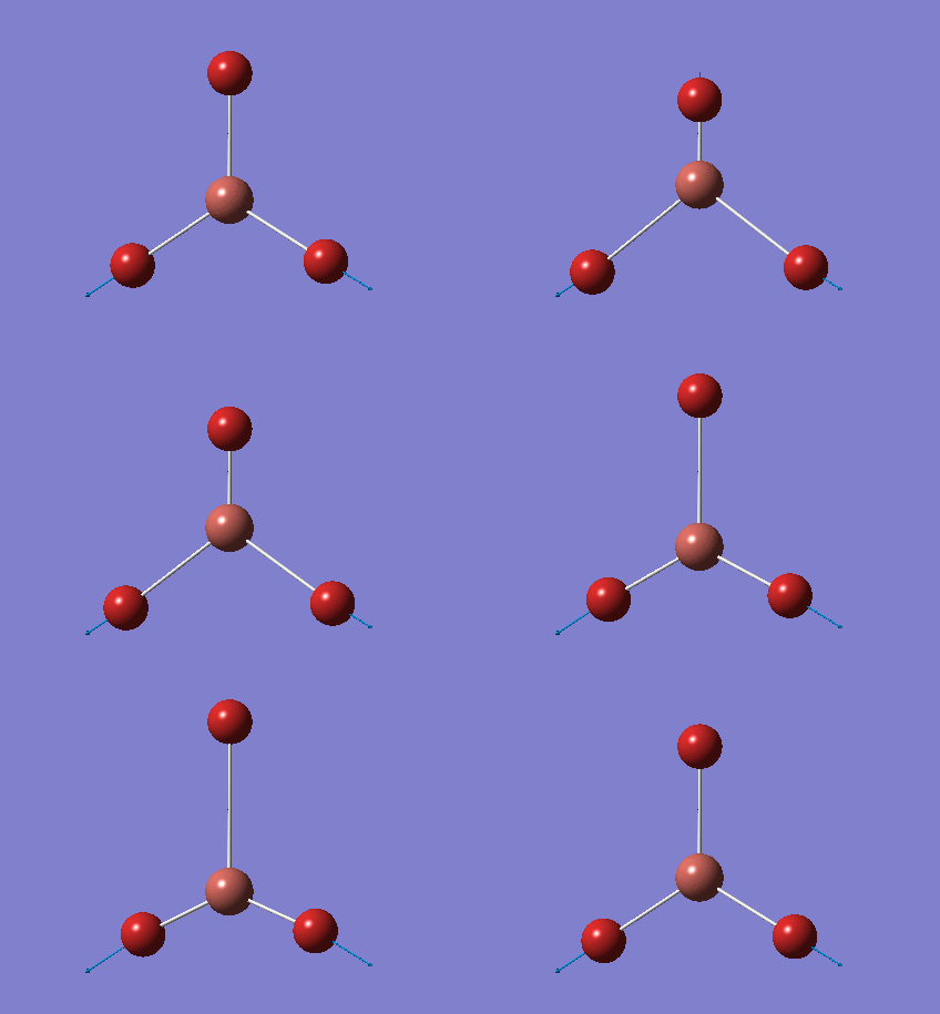
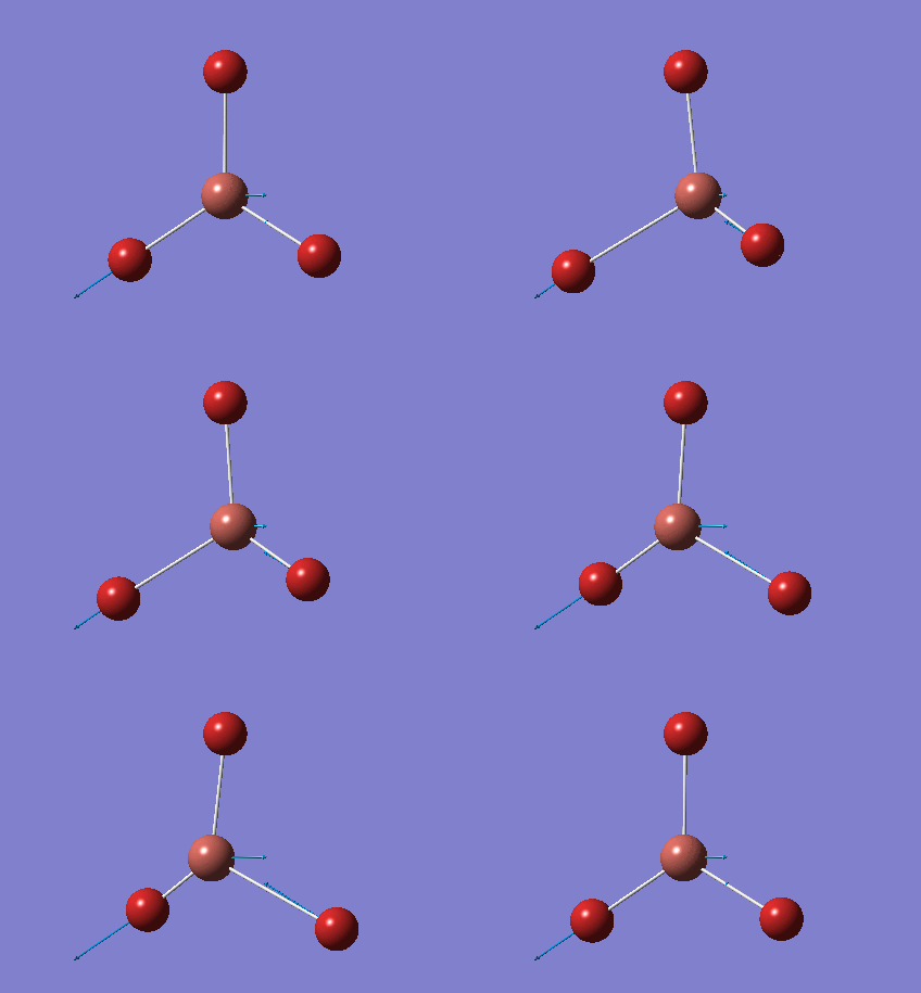
The lowest "real" normal mode is 50cm-1 with a E' symmetry label.
The list of absorptions are tabulated below:
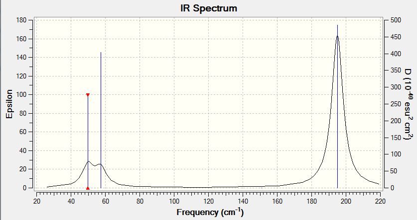
The IR spectrum is also shown:
The summary of the vibrations of the TlBr3 molecule:
Comparing the Absorption Frequencies of BH3 and TlBr3
Please see the following table for the comparison of the absorption frequencies estimated for the two optimsed molecules:
| BH3 (cm-1) | Absorption | TlBr3 (cm-1) | Absorption | |
|---|---|---|---|---|
| Absorption #1 | 1162.98cm-1 | 92.5497 | 49.98 | 3.4600 |
| Absorption #2 | 1213.17 | 14.0545 | 49.98 | 3.4600 |
| Absorption #3 | 1213.18 | 14.0581 | 57.46 | 5.8147 |
| Absorption #4 | 2582.32 | 0.0000 | 150.77 | 0.0000 |
| Absorption #5 | 2715.50 | 126.3285 | 195.01 | 23.6823 |
| Absorption #6 | 2715.50 | 126.3189 | 195.01 | 23.6845 |
From the data seen above, in general all absorptions in BH3 are much stronger than those in TlBr3, as reflected from the much higher wavenumbers, which correspond to energies (a higher wavenumber refers to a shorter wavelength and hence a higher energy level). This agrees with the prediction made in part 2.1.5 Summary and Comparison of BH3, BBr3, TlBr3 Bond Distances, which discussed the relative lengths and hence the energies of BH3 and TlBr3 bonds due to ortibal overlap. This in turn indicates that the B-H bonds are much stronger than the Tl-Br bonds.
These two IR spectra have a simliar shape, i.e. having two observable peaks on a lower wavenumber (c.a. 1200cm-1 for BH3 and c.a. 50cm-1 for TlBr3) and one observable peak (c.a. 2700cm-1 for BH3 and c.a. 195cm-1 for TlBr3) with a much higher intensity. The intensities of the absorptions of the two molecules, as reflected by the epsilon values, show that BH3 has much larger absorptions (larger epsilons) than Tl-Br3 due to stronger bonds, reasons explained in previous sections.
Questions:
- 1. Has there been a reordering of modes? The order of vibrations in BH3 and TlBr3 are reordered, possibly due to the different masses of the bonding atoms. The frequencies observed arise from different vibration modes, and the masses of the participating atoms can have significant effects. They vibrate in a different manner which corresponds to the frequencies observed.
- 2. For both spectra two modes lie fairly closely together, the A2 and E' modes and then the other two modes also lie fairly close together, the A1' and E' modes, but higher in energy. Why is this? The two vibrations with lower energy i.e. frequency correspond to bending vibrations, and the ones with higher energy refer to stretching vibrations which are higher energy vibrations in nature.
Discussion of the Frequency Analysis Process
The same method and basis set for both the optimisation and frequency analysis calculations were used. This is because the way Gaussian estimates the energy of a molecule is based on the accuracy of the basis sets and how the basis sets are arranged to mimic the molecular energy states. If different levels of accuracies of basis sets or the logarithm that the basis sets are arranged are different, the whole process will be different and the results yielded from these non-identical estimations are incomparable. We often need to refer to the energy estimation when we are analysing the absorptions of the molecule.
By carrying out a frequency analysis, Gaussian can predict different vibration modes the molecule possesses and hence can simulate the IR frequencies and the spectrum of the molecule. So the steps of analysis are as follows: first the molecule is set up in GaussView and a rough optimisation is carried out using a simplier basis set, this allows a rough estimation of the appropriate structure and coarsely tunes the structure of the molecule. The tuned molecule is then subjected to a finer and more accurate basis set using the same optimisation method and is more finely optimised. This takes a longer time but yields a more ideal molecule, with a lower energy and more realistic optimisation. This molecule is then subjected to frequency analysis, which predicts the vibration modes the molecule will adopt, and predicts the IR spectrum of the molecule, which can be compared to experimental data for further analysis.
The "Low frequencies", as mentioned as the part above, represent the "-6" part of 3N-6, which is defined as the degrees of freedom of the molecule. It refers to the number of physical states the molecule can adopt, so the smaller the value, the more accurate the estimation is, because it means that the estimated value is of a smaller range. A value larger than +-15 is generally unaccepted.
Evaluation of the MO energies of BH3
The MO energies of BH3 are estimated and the output .log uploaded to D-Space, link can be found here: [4]
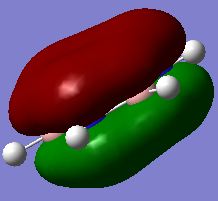
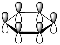
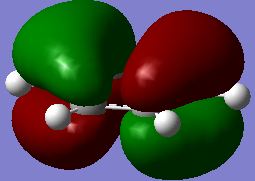
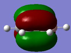
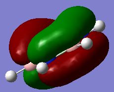
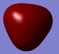
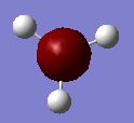
The predicted Molecular Orbitals (by linear combination of atomic orbitals) are also drawn using ChemDraw, which are then compared to the ones estimated using Gaussian. They are tabulated below:
| LCAO predicted | Gaussian simulated | |
|---|---|---|
| MO #5 (LUMO) | 
|
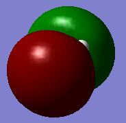
|
| MO #4 (HOMO) | 
|
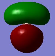
|
| MO #3 | 
|
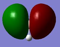
|
| MO #2 | 
|
|
| MO #1 | 
|
|
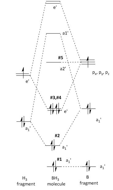
The MO diagram is showed below:
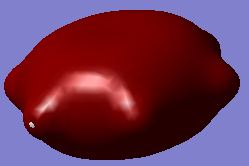
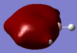
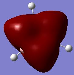
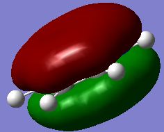
As seen in the table, the predicted and "real" MO's have the same shapes, and the real orbitals have electron density from orbitals of the same phase merged together. The "real" MO's are therefore a more realistic representation of the actual electron density distribution over the molecule, as in reality electrons circulate through the whole of the coloured regions, ignoring the space as shown in the LCAO predicted orbitals. But generally, the orbitals agree to a high level with the actual ones.
From this comparison it can be seen that qualitative MO (as reflected from the predicted MO by using the LCAO method) yields a very high level of agreement with that predicted using Gaussian. As can be seen from the comparison table above, all five orbitals match perfectly for the predicted and "actual, real" case. This shows that the LCAO prediction is reliable in predicting MO levels and orbital shapes and is a useful application.
Analysis on NH3
The NH3 molecule is set up and optimised:
- Optimisation method: B3LYP
- Optimisation basis set: 6-31G (d,p)
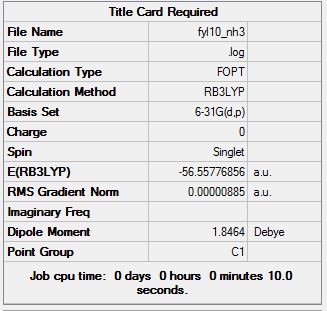
The .log file can be found here. The summary of the optimisation is shown:
And the Item section is included:
Item               Value     Threshold  Converged?
 Maximum Force            0.000024     0.000450     YES
 RMS     Force            0.000012     0.000300     YES
 Maximum Displacement     0.000079     0.001800     YES
 RMS     Displacement     0.000053     0.001200     YES
 Predicted change in Energy=-1.629728D-09
 Optimization completed.
    -- Stationary point found.
                           ----------------------------
                           !   Optimized Parameters   !
                           ! (Angstroms and Degrees)  !
 --------------------------                            --------------------------
 ! Name  Definition              Value          Derivative Info.                !
 --------------------------------------------------------------------------------
 ! R1    R(1,2)                  1.018          -DE/DX =    0.0                 !
 ! R2    R(1,3)                  1.018          -DE/DX =    0.0                 !
 ! R3    R(1,4)                  1.018          -DE/DX =    0.0                 !
 ! A1    A(2,1,3)              105.7413         -DE/DX =    0.0                 !
 ! A2    A(2,1,4)              105.7486         -DE/DX =    0.0                 !
 ! A3    A(3,1,4)              105.7479         -DE/DX =    0.0                 !
 ! D1    D(2,1,4,3)           -111.8631         -DE/DX =    0.0                 !
 --------------------------------------------------------------------------------
 GradGradGradGradGradGradGradGradGradGradGradGradGradGradGradGradGradGrad
With all values converging, and a gradient of 0.00000885 a.u. which is very small, the optimisation was successful and carried on to the next step.
The optimised molecule was then frequency-analysed and the .log can be found here: here
The Low Frequency section is included:
Low frequencies ---  -30.7764    0.0006    0.0013    0.0015   20.3142   28.2484
Low frequencies --- 1089.5557 1694.1237 1694.1868
The molecule was optimised two times to obtain this frequency analysis data. The largest deviation is -30.7764cm-1, which is quite large, but is the best value obtained from several attempts. The "real" frequencies are also all positive and valid for proceeding to the next step.
The IR spectrum and the absorptions are tabulated as below:
The molecule was also analysed to generate its molecular orbitals. The .log file of the energy analysis can be found here. The MO's obtained are shown:
| Gaussian simulated | |
|---|---|
| MO #6 (LUMO) | 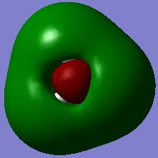
|
| MO #5 (HOMO) | 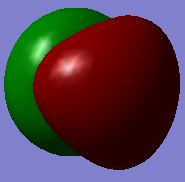
|
| MO #4 | 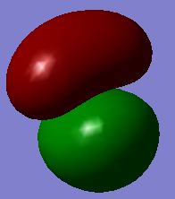
|
| MO #3 | 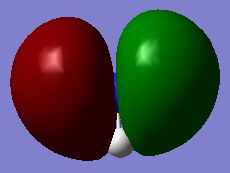
|
| MO #2 | 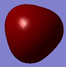
|
| MO #1 | 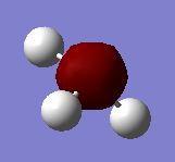
|
NBO analysis was then carried out on the energy-analysed file of NH3.
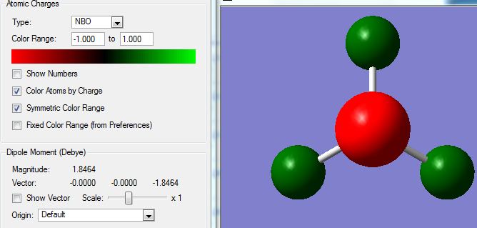
The charge on the molecule is shown below, the limits are from -1.00 to 1.00 with brightly red coloured orbitals highly negative and brightly green orbitals highly positive. The image is shown below:
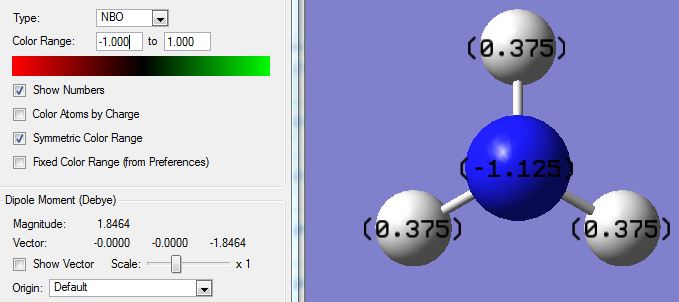
The numerical charges are also labelled, image as follows:
The numerical NBO charges are:
- Nitrogen: -1.125
- Oxygen: +0.375
Analysis of NH3BH3
Optimisation of the molecule
Optimisation conditions:
- Method: B3LYP
- Basis set: 6-31G (d,p)
The .log file can be found here: here
The summary is shown below:
The Item contents are shown:
Item               Value     Threshold  Converged?
 Maximum Force            0.000175     0.000450     YES
 RMS     Force            0.000075     0.000300     YES
 Maximum Displacement     0.000695     0.001800     YES
 RMS     Displacement     0.000334     0.001200     YES
 Predicted change in Energy=-2.601134D-07
 Optimization completed.
    -- Stationary point found.
                           ----------------------------
                           !   Optimized Parameters   !
                           ! (Angstroms and Degrees)  !
 --------------------------                            --------------------------
 ! Name  Definition              Value          Derivative Info.                !
 --------------------------------------------------------------------------------
 ! R1    R(1,7)                  1.0176         -DE/DX =   -0.0002              !
 ! R2    R(2,7)                  1.0176         -DE/DX =   -0.0002              !
 ! R3    R(3,7)                  1.0176         -DE/DX =   -0.0002              !
 ! R4    R(4,8)                  1.2084         -DE/DX =   -0.0001              !
 ! R5    R(5,8)                  1.2084         -DE/DX =   -0.0001              !
 ! R6    R(6,8)                  1.2084         -DE/DX =   -0.0001              !
 ! R7    R(7,8)                  1.6637         -DE/DX =   -0.0001              !
 ! A1    A(1,7,2)              107.7966         -DE/DX =    0.0                 !
 ! A2    A(1,7,3)              107.7985         -DE/DX =    0.0                 !
 ! A3    A(1,7,8)              111.0986         -DE/DX =    0.0                 !
 ! A4    A(2,7,3)              107.7946         -DE/DX =    0.0                 !
 ! A5    A(2,7,8)              111.0978         -DE/DX =    0.0                 !
 ! A6    A(3,7,8)              111.0977         -DE/DX =    0.0                 !
 ! A7    A(4,8,5)              113.6415         -DE/DX =    0.0                 !
 ! A8    A(4,8,6)              113.6398         -DE/DX =    0.0                 !
 ! A9    A(4,8,7)              104.8852         -DE/DX =    0.0                 !
 ! A10   A(5,8,6)              113.6383         -DE/DX =    0.0                 !
 ! A11   A(5,8,7)              104.8916         -DE/DX =    0.0                 !
 ! A12   A(6,8,7)              104.8857         -DE/DX =    0.0                 !
 ! D1    D(1,7,8,4)            179.9988         -DE/DX =    0.0                 !
 ! D2    D(1,7,8,5)            -59.9986         -DE/DX =    0.0                 !
 ! D3    D(1,7,8,6)             60.0007         -DE/DX =    0.0                 !
 ! D4    D(2,7,8,4)            -60.001          -DE/DX =    0.0                 !
 ! D5    D(2,7,8,5)             60.0017         -DE/DX =    0.0                 !
 ! D6    D(2,7,8,6)            180.001          -DE/DX =    0.0                 !
 ! D7    D(3,7,8,4)             59.9961         -DE/DX =    0.0                 !
 ! D8    D(3,7,8,5)           -180.0012         -DE/DX =    0.0                 !
 ! D9    D(3,7,8,6)            -60.0019         -DE/DX =    0.0                 !
 --------------------------------------------------------------------------------
 GradGradGradGradGradGradGradGradGradGradGradGradGradGradGradGradGradGrad
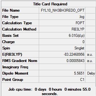
Having all converging values and the gradient being 0.00005843, which is reasonably small, the optimisation is taken to be valid and moved on to frequency analysis.
Frequency Analysis
The analysed .log file can be found here:here
The LOW FREQUENCY list is shown:
Low frequencies ---   -0.0008    0.0004    0.0006   19.5407   24.0603   39.4387
 Low frequencies ---  278.5908  636.9484  654.7447
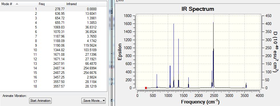
The IR spectrum and absorptions are shown below:
It can be seen from the IR analysis data that the highest "low frequency" is +39 which is quite large (usually +-15 is the acceptable range). However, the same action, i.e. optimisation followed by frequency analysis was completed several times and this is the best value obtained. There are no negative real frequencies and the analysis is carried on. However, the deviation is quite significant compared to the smallest "real frequency" of 279cm-1, with a percentage error of approximately 10%.
Comparison of BH3, NH3 and NH3BH3 Molecular Energies
Summary of calculated energies of the molecules:
- E(BH3)= -26.61532252 a.u.
- E(NH3)= -56.55776845 a.u.
- E(NH3BH3)= -83.22468956 a.u.
Difference in energy:
ΔE=E(NH3BH3)-[E(NH3)+E(BH3)]
=-83.22468956 - (-56.55776845-26.61532252) =-0.05159699 a.u.
=-135.467897kJ/mol, the association energy of joining a BH3 and a NH3 to form a NH3BH3 molecule.
Week 2: Mini Project - Aromaticity
The common aromatic molecule, benzene C6H6, is optimised analysed using computational calculations. Frequency, population and NBO analyses were carried out for this molecule using the HPC server. Its isoelectronic analogues, boratabenzene (one C replaced by a B with a negative charge), and pyridinium (one C replaced by a N with a positive charge) are also analysed in the same way using the same method and compared to the benzene analysis results, to investigate the properties of these aromatic compounds.
Investigating Benzene
Optimisation
A benzene molecule was set up in GaussView and optimised on the HPC server, the .log file can be found here at [5].
- Job type: OPT
- Method: B3YLP
- Basis set: 6-31G(d,p)
The summary of the optimisation is shown:
The Items content is also shown:
Item               Value     Threshold  Converged?
 Maximum Force            0.000212     0.000450     YES
 RMS     Force            0.000085     0.000300     YES
 Maximum Displacement     0.000991     0.001800     YES
 RMS     Displacement     0.000315     0.001200     YES
 Predicted change in Energy=-5.157454D-07
 Optimization completed.
    -- Stationary point found.
                           ----------------------------
                           !   Optimized Parameters   !
                           ! (Angstroms and Degrees)  !
 --------------------------                            --------------------------
 ! Name  Definition              Value          Derivative Info.                !
 --------------------------------------------------------------------------------
 ! R1    R(1,2)                  1.3963         -DE/DX =    0.0001              !
 ! R2    R(1,6)                  1.3961         -DE/DX =    0.0002              !
 ! R3    R(1,7)                  1.0861         -DE/DX =    0.0002              !
 ! R4    R(2,3)                  1.3961         -DE/DX =    0.0002              !
 ! R5    R(2,8)                  1.0861         -DE/DX =    0.0002              !
 ! R6    R(3,4)                  1.3963         -DE/DX =    0.0001              !
 ! R7    R(3,9)                  1.086          -DE/DX =    0.0002              !
 ! R8    R(4,5)                  1.3961         -DE/DX =    0.0002              !
 ! R9    R(4,10)                 1.086          -DE/DX =    0.0002              !
 ! R10   R(5,6)                  1.3963         -DE/DX =    0.0001              !
 ! R11   R(5,11)                 1.0861         -DE/DX =    0.0002              !
 ! R12   R(6,12)                 1.0861         -DE/DX =    0.0002              !
 ! A1    A(2,1,6)              119.9972         -DE/DX =    0.0                 !
 ! A2    A(2,1,7)              119.9949         -DE/DX =    0.0                 !
 ! A3    A(6,1,7)              120.0079         -DE/DX =    0.0                 !
 ! A4    A(1,2,3)              120.0079         -DE/DX =    0.0                 !
 ! A5    A(1,2,8)              119.9881         -DE/DX =    0.0                 !
 ! A6    A(3,2,8)              120.004          -DE/DX =    0.0                 !
 ! A7    A(2,3,4)              119.9948         -DE/DX =    0.0                 !
 ! A8    A(2,3,9)              120.0086         -DE/DX =    0.0                 !
 ! A9    A(4,3,9)              119.9966         -DE/DX =    0.0                 !
 ! A10   A(3,4,5)              119.9972         -DE/DX =    0.0                 !
 ! A11   A(3,4,10)             119.9934         -DE/DX =    0.0                 !
 ! A12   A(5,4,10)             120.0094         -DE/DX =    0.0                 !
 ! A13   A(4,5,6)              120.0083         -DE/DX =    0.0                 !
 ! A14   A(4,5,11)             120.0014         -DE/DX =    0.0                 !
 ! A15   A(6,5,11)             119.9904         -DE/DX =    0.0                 !
 ! A16   A(1,6,5)              119.9946         -DE/DX =    0.0                 !
 ! A17   A(1,6,12)             120.0106         -DE/DX =    0.0                 !
 ! A18   A(5,6,12)             119.9948         -DE/DX =    0.0                 !
 ! D1    D(6,1,2,3)             -0.0059         -DE/DX =    0.0                 !
 ! D2    D(6,1,2,8)            180.0023         -DE/DX =    0.0                 !
 ! D3    D(7,1,2,3)           -180.01           -DE/DX =    0.0                 !
 ! D4    D(7,1,2,8)             -0.0019         -DE/DX =    0.0                 !
 ! D5    D(2,1,6,5)             -0.0055         -DE/DX =    0.0                 !
 ! D6    D(2,1,6,12)          -179.9972         -DE/DX =    0.0                 !
 ! D7    D(7,1,6,5)           -180.0013         -DE/DX =    0.0                 !
 ! D8    D(7,1,6,12)             0.007          -DE/DX =    0.0                 !
 ! D9    D(1,2,3,4)              0.0117         -DE/DX =    0.0                 !
 ! D10   D(1,2,3,9)           -179.9914         -DE/DX =    0.0                 !
 ! D11   D(8,2,3,4)            180.0036         -DE/DX =    0.0                 !
 ! D12   D(8,2,3,9)              0.0005         -DE/DX =    0.0                 !
 ! D13   D(2,3,4,5)             -0.0062         -DE/DX =    0.0                 !
 ! D14   D(2,3,4,10)          -180.0059         -DE/DX =    0.0                 !
 ! D15   D(9,3,4,5)            179.9969         -DE/DX =    0.0                 !
 ! D16   D(9,3,4,10)            -0.0028         -DE/DX =    0.0                 !
 ! D17   D(3,4,5,6)             -0.0051         -DE/DX =    0.0                 !
 ! D18   D(3,4,5,11)           180.0058         -DE/DX =    0.0                 !
 ! D19   D(10,4,5,6)          -180.0055         -DE/DX =    0.0                 !
 ! D20   D(10,4,5,11)            0.0054         -DE/DX =    0.0                 !
 ! D21   D(4,5,6,1)              0.011          -DE/DX =    0.0                 !
 ! D22   D(4,5,6,12)           180.0027         -DE/DX =    0.0                 !
 ! D23   D(11,5,6,1)          -179.9999         -DE/DX =    0.0                 !
 ! D24   D(11,5,6,12)           -0.0082         -DE/DX =    0.0                 !
 --------------------------------------------------------------------------------
 GradGradGradGradGradGradGradGradGradGradGradGradGradGradGradGradGradGrad
Having all converging values, and a gradient of 0.00009549 a.u. which is reasonably small, the optimisation is proved to be valid and is moved on to frequency analysis.
Frequency Analysis
Using the optimised .log file, a frequency analysis was carried out, the resulting files were uploaded and can be found here at [6].
The LOW FREQUENCIES can also be found here:
Low frequencies ---  -17.2788  -14.5868   -9.6527    0.0009    0.0012    0.0012
 Low frequencies ---  413.7971  414.4697  620.8545
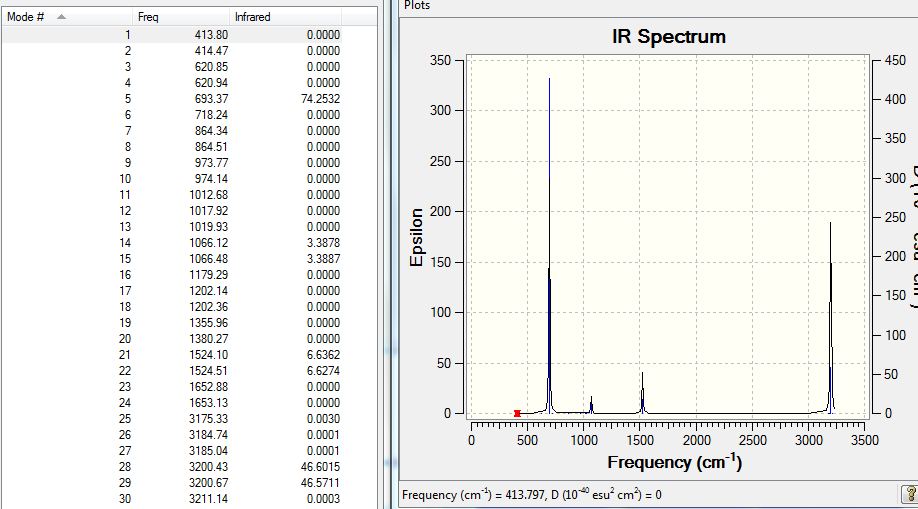
Having a max low frequency of -17cm-1 it is not a small value, but it still lies within an acceptable range.
The list of absorptions are included for reference:
Population and NBO Analysis
Using the optimised .chk file, an energy calculation was carried out and the file uploaded to D-Space and can be found here at [7]
- Job type: Energy
- Additional keywords: pop=full
- NBO type: Full NBO
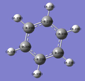
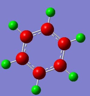
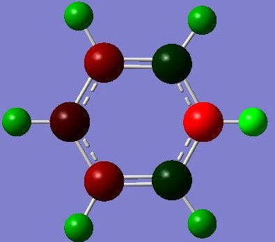
The NBO analysis of the molecule also showed the charge distribution on the C and H atoms as expected due to a larger electronegativity for C atoms. Images are shown below:
Displaying numbers:
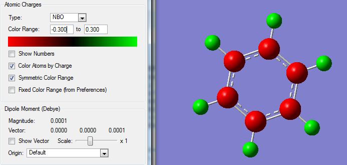
Displaying coloured charges: (from bright red at -0.300 to bright green at +0.300)
MO Diagram and Analysis
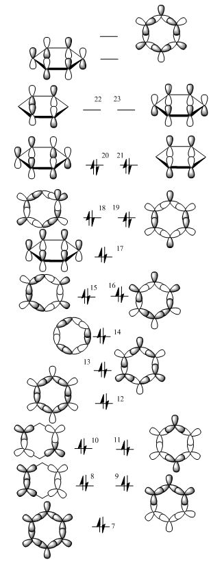
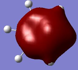
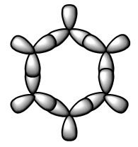
The .log file from energy analysis of benzene was examined and the MO's were visualised in GaussView. The "centre" part of the MO diagram was constructed from the visualised MO generated by GaussView. The predicted MO diagram is shown below:
Description of the MO diagram: Starting from the seventh MO, the electron density is spread over the whole molecule. The first to the sixth orbitals are concerned only with the carbon atoms, and are combinations of the carbon 1s orbitals which are "core" and not interesting to this project. The LCAO of atomic 2s and 2p orbitals are simulated from the MO calculation generated from the population analysis of the optimised molecule. As we can see, the number of nodes in the MO's increases for higher level MO's, leading to a higher energy combination. The carbon p orbitals perpendicular to the plane of the benzene molecule have higher energy levels, and are found as MO's 17 and 20-23. All resulting MO's of the molecule up to the LUMO (the degenerate 22nd and 23rd MO's) are predicted, other than the core (first to sixth MO's) orbitals.
Relation of MO's to aromaticity: The MO diagram generated contains orbitals involving the LCAO of BOTH p orbitals from carbon (which are the ones usually considered when referring to aromatic compounds), and also s orbitals from hydrogen atoms and carbon atoms. The LCAO of these orbitals formed the basis of the MO diagram shown. As for connection to aromaticity of benzene, LCAO of the 2p carbon orbitals which are perpendicular to the plane of the benzene molecule are the ones involved, contributing to the stabilising effect of the molecule, as known as aromaticity. The MO's labelled #17, #20, #21, #22, #23 and the MO second highest in energy shown in the MO diagram contribute to the aromaticity of the molecule, having three of the six orbitals filled with 2 electrons each, having 6 electrons in the MO formed by LCAO of the p-orbitals. Huckel aromaticity applies to molecules with 2n+2 (n is an integer) electrons. In benzene, the 6 electrons from MO's #17, #20 and #21 fulfills the 2n+2 requirement with n=2, which chemically represents the delocalisation of the 6 electrons into the ring formed by the 6 carbon atoms the MO's are based on. These delocalised pi-electrons generate a magnetic ring current and stabilise atoms within the vicinity of the current.
Boratabenzene
Optimisation
File uploaded to D-Space and link found here [8].
- Job type: OPT
- Method: B3LYP
- Basis set: 6-31G(d,p)
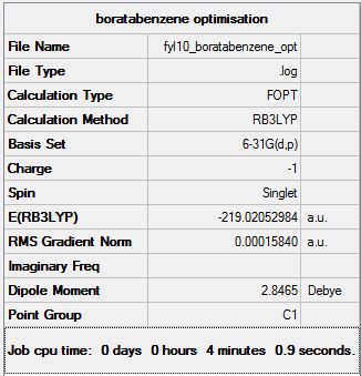
The summary table is uploaded:
The Items table is also included:
Item               Value     Threshold  Converged?
 Maximum Force            0.000159     0.000450     YES
 RMS     Force            0.000069     0.000300     YES
 Maximum Displacement     0.000878     0.001800     YES
 RMS     Displacement     0.000326     0.001200     YES
 Predicted change in Energy=-6.589451D-07
 Optimization completed.
    -- Stationary point found.
                           ----------------------------
                           !   Optimized Parameters   !
                           ! (Angstroms and Degrees)  !
 --------------------------                            --------------------------
 ! Name  Definition              Value          Derivative Info.                !
 --------------------------------------------------------------------------------
 ! R1    R(1,2)                  1.4053         -DE/DX =   -0.0001              !
 ! R2    R(1,5)                  1.3989         -DE/DX =    0.0                 !
 ! R3    R(1,6)                  1.0968         -DE/DX =    0.0001              !
 ! R4    R(2,3)                  1.4053         -DE/DX =   -0.0001              !
 ! R5    R(2,7)                  1.0916         -DE/DX =   -0.0001              !
 ! R6    R(3,4)                  1.3989         -DE/DX =    0.0                 !
 ! R7    R(3,8)                  1.0968         -DE/DX =    0.0001              !
 ! R8    R(4,9)                  1.097          -DE/DX =   -0.0001              !
 ! R9    R(4,12)                 1.5137         -DE/DX =    0.0001              !
 ! R10   R(5,11)                 1.097          -DE/DX =   -0.0001              !
 ! R11   R(5,12)                 1.5138         -DE/DX =    0.0001              !
 ! R12   R(10,12)                1.2185         -DE/DX =    0.0                 !
 ! A1    A(2,1,5)              122.138          -DE/DX =    0.0001              !
 ! A2    A(2,1,6)              117.4354         -DE/DX =    0.0                 !
 ! A3    A(5,1,6)              120.4266         -DE/DX =   -0.0002              !
 ! A4    A(1,2,3)              120.4508         -DE/DX =   -0.0001              !
 ! A5    A(1,2,7)              119.7734         -DE/DX =    0.0001              !
 ! A6    A(3,2,7)              119.7758         -DE/DX =    0.0001              !
 ! A7    A(2,3,4)              122.1395         -DE/DX =    0.0001              !
 ! A8    A(2,3,8)              117.4371         -DE/DX =    0.0                 !
 ! A9    A(4,3,8)              120.4234         -DE/DX =   -0.0002              !
 ! A10   A(3,4,9)              115.9493         -DE/DX =    0.0001              !
 ! A11   A(3,4,12)             120.0806         -DE/DX =   -0.0001              !
 ! A12   A(9,4,12)             123.9701         -DE/DX =   -0.0001              !
 ! A13   A(1,5,11)             115.9535         -DE/DX =    0.0001              !
 ! A14   A(1,5,12)             120.0812         -DE/DX =   -0.0001              !
 ! A15   A(11,5,12)            123.9654         -DE/DX =   -0.0001              !
 ! A16   A(4,12,5)             115.1098         -DE/DX =    0.0                 !
 ! A17   A(4,12,10)            122.4482         -DE/DX =    0.0                 !
 ! A18   A(5,12,10)            122.4419         -DE/DX =    0.0                 !
 ! D1    D(5,1,2,3)              0.0057         -DE/DX =    0.0                 !
 ! D2    D(5,1,2,7)            180.0027         -DE/DX =    0.0                 !
 ! D3    D(6,1,2,3)            180.0038         -DE/DX =    0.0                 !
 ! D4    D(6,1,2,7)              0.0008         -DE/DX =    0.0                 !
 ! D5    D(2,1,5,11)          -180.0018         -DE/DX =    0.0                 !
 ! D6    D(2,1,5,12)            -0.001          -DE/DX =    0.0                 !
 ! D7    D(6,1,5,11)             0.0002         -DE/DX =    0.0                 !
 ! D8    D(6,1,5,12)           180.001          -DE/DX =    0.0                 !
 ! D9    D(1,2,3,4)             -0.0074         -DE/DX =    0.0                 !
 ! D10   D(1,2,3,8)           -180.0016         -DE/DX =    0.0                 !
 ! D11   D(7,2,3,4)           -180.0044         -DE/DX =    0.0                 !
 ! D12   D(7,2,3,8)              0.0014         -DE/DX =    0.0                 !
 ! D13   D(2,3,4,9)            180.0049         -DE/DX =    0.0                 !
 ! D14   D(2,3,4,12)             0.0042         -DE/DX =    0.0                 !
 ! D15   D(8,3,4,9)             -0.0011         -DE/DX =    0.0                 !
 ! D16   D(8,3,4,12)          -180.0018         -DE/DX =    0.0                 !
 ! D17   D(3,4,12,5)             0.0005         -DE/DX =    0.0                 !
 ! D18   D(3,4,12,10)         -180.0            -DE/DX =    0.0                 !
 ! D19   D(9,4,12,5)          -180.0003         -DE/DX =    0.0                 !
 ! D20   D(9,4,12,10)           -0.0008         -DE/DX =    0.0                 !
 ! D21   D(1,5,12,4)            -0.002          -DE/DX =    0.0                 !
 ! D22   D(1,5,12,10)         -180.0015         -DE/DX =    0.0                 !
 ! D23   D(11,5,12,4)          179.9989         -DE/DX =    0.0                 !
 ! D24   D(11,5,12,10)          -0.0006         -DE/DX =    0.0                 !
 --------------------------------------------------------------------------------
 GradGradGradGradGradGradGradGradGradGradGradGradGradGradGradGradGradGrad
All converging values for the optimisation and a small gradient of 0.00015840 a.u. shows that optimisation is complete. Moved on to frequency and energy analysis.
Frequency Analysis
The same method and basis sets were used, results file uploaded to D-Space and can be found here: [9].
The low frequencies lines were reported:
Low frequencies ---  -13.1275   -0.0007    0.0007    0.0007   15.0447   18.1653
 Low frequencies ---  371.3454  404.2334  565.2534
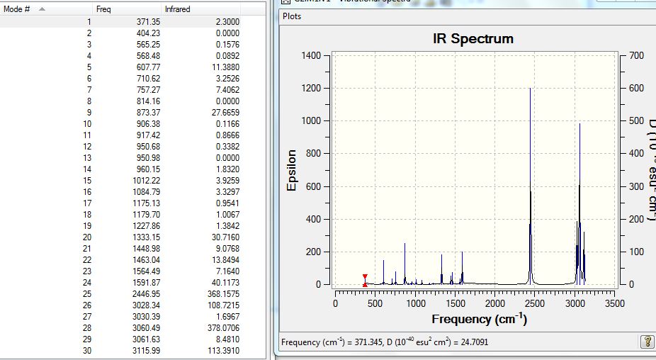
The largest low frequency is 18cm-1, which is a bit large but reasonable. Having no negative real frequencies also confirmed the success of this frequency analysis. A list of the absorptions for this molecule is also included:
Population and NBO Analysis
The .chk file after optimisation was population-analysed and uploaded to the D-Space server, the link can be found here: [10].
- Job type: Energy
- Additional keywords: pop=full
- NBO type: Full NBO
The NBO Analysis of the molecule was also processed and images posted:
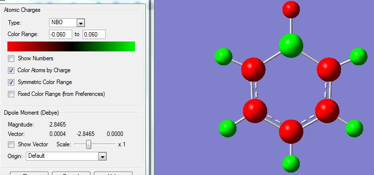
Showing coloured atoms (green refers to a positive charge and red a negative charge, from -0.060 to +0.060):
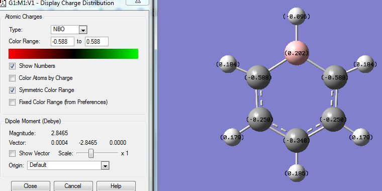
Showing numbered charges:
As expected from the atomic electronegativities of C (2.5), B(2.0), H(2.1), the atomic charges in increasing negative charge follow the trend of B < H < C. The carbon atoms ortho- to the electropositive boron atom have a higher negative charge compared to the carbons on the meta- and para- positions, since C has a higher electronegativity than B, the B atom donates electron density to the neighbouring (ortho-) carbon atoms leading to this observation.
Pyridinium
Optimisation
The optimisation is carried on the HPC server and uploaded to D-Space, link can be found here: [11].
- Job type: OPT
- Method: B3LYP
- Basis set: 6-31G(d,p)
The summary table is included:
The Items table is also shown:
Item               Value     Threshold  Converged?
 Maximum Force            0.000065     0.000450     YES
 RMS     Force            0.000023     0.000300     YES
 Maximum Displacement     0.000826     0.001800     YES
 RMS     Displacement     0.000176     0.001200     YES
 Predicted change in Energy=-6.972574D-08
 Optimization completed.
    -- Stationary point found.
                           ----------------------------
                           !   Optimized Parameters   !
                           ! (Angstroms and Degrees)  !
 --------------------------                            --------------------------
 ! Name  Definition              Value          Derivative Info.                !
 --------------------------------------------------------------------------------
 ! R1    R(1,2)                  1.3988         -DE/DX =    0.0                 !
 ! R2    R(1,5)                  1.3838         -DE/DX =    0.0                 !
 ! R3    R(1,6)                  1.0835         -DE/DX =    0.0                 !
 ! R4    R(2,3)                  1.3988         -DE/DX =    0.0                 !
 ! R5    R(2,7)                  1.0852         -DE/DX =    0.0                 !
 ! R6    R(3,4)                  1.3839         -DE/DX =    0.0                 !
 ! R7    R(3,8)                  1.0835         -DE/DX =    0.0                 !
 ! R8    R(4,9)                  1.0832         -DE/DX =    0.0                 !
 ! R9    R(4,12)                 1.3523         -DE/DX =    0.0001              !
 ! R10   R(5,11)                 1.0832         -DE/DX =    0.0                 !
 ! R11   R(5,12)                 1.3524         -DE/DX =    0.0                 !
 ! R12   R(10,12)                1.0169         -DE/DX =    0.0                 !
 ! A1    A(2,1,5)              119.0827         -DE/DX =    0.0                 !
 ! A2    A(2,1,6)              121.496          -DE/DX =   -0.0001              !
 ! A3    A(5,1,6)              119.4213         -DE/DX =    0.0                 !
 ! A4    A(1,2,3)              120.0549         -DE/DX =    0.0                 !
 ! A5    A(1,2,7)              119.9711         -DE/DX =    0.0                 !
 ! A6    A(3,2,7)              119.974          -DE/DX =    0.0                 !
 ! A7    A(2,3,4)              119.082          -DE/DX =    0.0                 !
 ! A8    A(2,3,8)              121.4988         -DE/DX =   -0.0001              !
 ! A9    A(4,3,8)              119.4192         -DE/DX =    0.0001              !
 ! A10   A(3,4,9)              123.9297         -DE/DX =    0.0                 !
 ! A11   A(3,4,12)             119.2363         -DE/DX =    0.0                 !
 ! A12   A(9,4,12)             116.834          -DE/DX =    0.0                 !
 ! A13   A(1,5,11)             123.9327         -DE/DX =    0.0                 !
 ! A14   A(1,5,12)             119.2354         -DE/DX =    0.0                 !
 ! A15   A(11,5,12)            116.8319         -DE/DX =    0.0                 !
 ! A16   A(4,12,5)             123.3088         -DE/DX =    0.0                 !
 ! A17   A(4,12,10)            118.3463         -DE/DX =    0.0                 !
 ! A18   A(5,12,10)            118.345          -DE/DX =    0.0                 !
 ! D1    D(5,1,2,3)              0.0006         -DE/DX =    0.0                 !
 ! D2    D(5,1,2,7)           -180.0023         -DE/DX =    0.0                 !
 ! D3    D(6,1,2,3)            180.0015         -DE/DX =    0.0                 !
 ! D4    D(6,1,2,7)             -0.0014         -DE/DX =    0.0                 !
 ! D5    D(2,1,5,11)          -180.0005         -DE/DX =    0.0                 !
 ! D6    D(2,1,5,12)             0.0021         -DE/DX =    0.0                 !
 ! D7    D(6,1,5,11)            -0.0014         -DE/DX =    0.0                 !
 ! D8    D(6,1,5,12)           180.0012         -DE/DX =    0.0                 !
 ! D9    D(1,2,3,4)             -0.0024         -DE/DX =    0.0                 !
 ! D10   D(1,2,3,8)           -180.0018         -DE/DX =    0.0                 !
 ! D11   D(7,2,3,4)            180.0005         -DE/DX =    0.0                 !
 ! D12   D(7,2,3,8)              0.0012         -DE/DX =    0.0                 !
 ! D13   D(2,3,4,9)            180.0002         -DE/DX =    0.0                 !
 ! D14   D(2,3,4,12)             0.0015         -DE/DX =    0.0                 !
 ! D15   D(8,3,4,9)             -0.0004         -DE/DX =    0.0                 !
 ! D16   D(8,3,4,12)           180.0008         -DE/DX =    0.0                 !
 ! D17   D(3,4,12,5)             0.0014         -DE/DX =    0.0                 !
 ! D18   D(3,4,12,10)         -180.001          -DE/DX =    0.0                 !
 ! D19   D(9,4,12,5)           180.0025         -DE/DX =    0.0                 !
 ! D20   D(9,4,12,10)            0.0001         -DE/DX =    0.0                 !
 ! D21   D(1,5,12,4)            -0.0032         -DE/DX =    0.0                 !
 ! D22   D(1,5,12,10)         -180.0008         -DE/DX =    0.0                 !
 ! D23   D(11,5,12,4)         -180.0007         -DE/DX =    0.0                 !
 ! D24   D(11,5,12,10)           0.0016         -DE/DX =    0.0                 !
 --------------------------------------------------------------------------------
 GradGradGradGradGradGradGradGradGradGradGradGradGradGradGradGradGradGrad
Having all four converging values and a gradient of 0.00003894 a.u. the optimisation is properly done.
Frequency Analysis
Frequency analysis was carried out and the file can be found here: [12].
The LOW FREQUENCIES part is also shown:
Low frequencies ---   -7.2115   -0.0006    0.0009    0.0009   17.3444   18.5499
 Low frequencies ---  392.4572  404.0614  620.4717
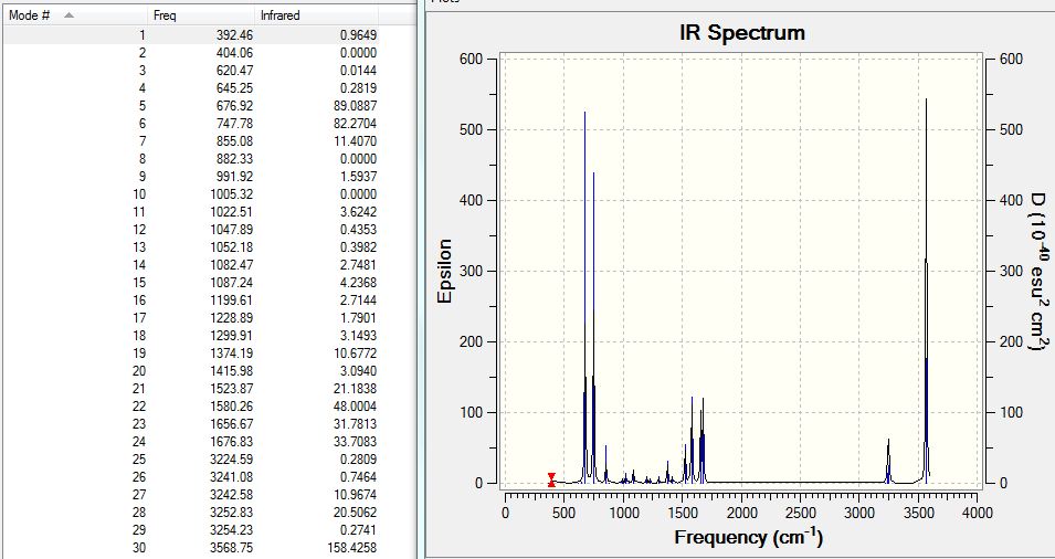
The largest low frequency is 19cm-1 which is quite large but acceptable. Having no negative real frequencies the analysis is taken to be valid and carried on to the next step.
The IR absorptions and spectrum are also shown:
Population and NBO Analysis
The .chk file of the optimised molecule was submitted to HPC and the resulting .log file can be found here on D-Space: [13].
- Job type: Energy
- Additional keywords: pop=full
- NBO type: Full NBO
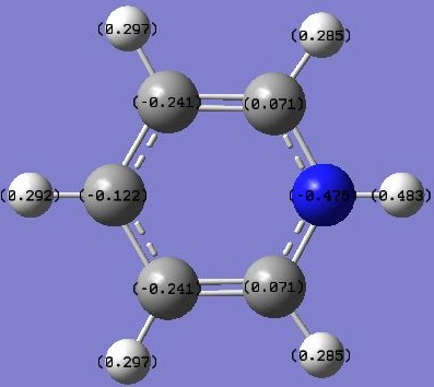
The NBO Analysis of the molecule was also processed and images posted:
Showing coloured atoms (green means positively charges and red negatively charged):
Showing numbered charges:
As expected, the charges residing on atoms are directly affected by the electronegativity of the atoms. N(3.0), C(2.5), H(2.1), therefore the N atom is the most negatively charged, followed by carbon atoms. Hydrogen atoms are the most positively charged. From the numbered NBO image, it can also be seen that the carbon atoms ortho- to the electronegative N atom are more positively charged than the meta- and para- carbons, as expected, due to the electron density on these carbon atoms are closer to the electronegative N atom and are directed away from the less electronegative carbon atoms, leading to a more positive charge.
Borazine
Optimisation
The optimisation is carried on the HPC server and uploaded to D-Space, link can be found here: [14].
- Job type: OPT
- Method: B3LYP
- Basis set: 6-31G(d,p)
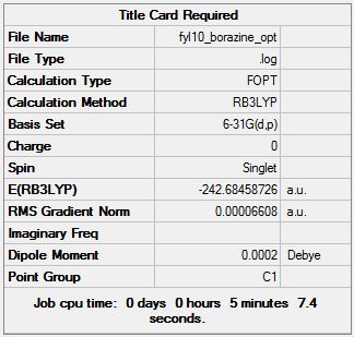
The summary table is shown:
The Items table is also shown:
Item               Value     Threshold  Converged?
 Maximum Force            0.000093     0.000450     YES
 RMS     Force            0.000033     0.000300     YES
 Maximum Displacement     0.000341     0.001800     YES
 RMS     Displacement     0.000096     0.001200     YES
 Predicted change in Energy=-1.028633D-07
 Optimization completed.
    -- Stationary point found.
                           ----------------------------
                           !   Optimized Parameters   !
                           ! (Angstroms and Degrees)  !
 --------------------------                            --------------------------
 ! Name  Definition              Value          Derivative Info.                !
 --------------------------------------------------------------------------------
 ! R1    R(1,9)                  1.1949         -DE/DX =    0.0001              !
 ! R2    R(2,12)                 1.0097         -DE/DX =    0.0                 !
 ! R3    R(3,8)                  1.1949         -DE/DX =    0.0001              !
 ! R4    R(4,10)                 1.0097         -DE/DX =    0.0                 !
 ! R5    R(5,7)                  1.1949         -DE/DX =    0.0001              !
 ! R6    R(6,11)                 1.0097         -DE/DX =    0.0                 !
 ! R7    R(7,10)                 1.4306         -DE/DX =   -0.0001              !
 ! R8    R(7,11)                 1.4307         -DE/DX =   -0.0001              !
 ! R9    R(8,10)                 1.4307         -DE/DX =   -0.0001              !
 ! R10   R(8,12)                 1.4307         -DE/DX =    0.0                 !
 ! R11   R(9,11)                 1.4306         -DE/DX =    0.0                 !
 ! R12   R(9,12)                 1.4307         -DE/DX =    0.0                 !
 ! A1    A(5,7,10)             121.4436         -DE/DX =    0.0                 !
 ! A2    A(5,7,11)             121.4373         -DE/DX =    0.0                 !
 ! A3    A(10,7,11)            117.119          -DE/DX =    0.0001              !
 ! A4    A(3,8,10)             121.4337         -DE/DX =    0.0                 !
 ! A5    A(3,8,12)             121.4348         -DE/DX =    0.0                 !
 ! A6    A(10,8,12)            117.1314         -DE/DX =    0.0                 !
 ! A7    A(1,9,11)             121.4414         -DE/DX =    0.0                 !
 ! A8    A(1,9,12)             121.4399         -DE/DX =    0.0                 !
 ! A9    A(11,9,12)            117.1187         -DE/DX =    0.0                 !
 ! A10   A(4,10,7)             118.567          -DE/DX =    0.0                 !
 ! A11   A(4,10,8)             118.5613         -DE/DX =    0.0                 !
 ! A12   A(7,10,8)             122.8717         -DE/DX =    0.0                 !
 ! A13   A(6,11,7)             118.5563         -DE/DX =    0.0                 !
 ! A14   A(6,11,9)             118.5584         -DE/DX =    0.0                 !
 ! A15   A(7,11,9)             122.8853         -DE/DX =    0.0                 !
 ! A16   A(2,12,8)             118.5639         -DE/DX =    0.0                 !
 ! A17   A(2,12,9)             118.5622         -DE/DX =    0.0                 !
 ! A18   A(8,12,9)             122.8739         -DE/DX =    0.0                 !
 ! D1    D(5,7,10,4)             0.0043         -DE/DX =    0.0                 !
 ! D2    D(5,7,10,8)          -179.9997         -DE/DX =    0.0                 !
 ! D3    D(11,7,10,4)         -179.9957         -DE/DX =    0.0                 !
 ! D4    D(11,7,10,8)            0.0002         -DE/DX =    0.0                 !
 ! D5    D(5,7,11,6)             0.0003         -DE/DX =    0.0                 !
 ! D6    D(5,7,11,9)           179.9967         -DE/DX =    0.0                 !
 ! D7    D(10,7,11,6)         -179.9996         -DE/DX =    0.0                 !
 ! D8    D(10,7,11,9)           -0.0033         -DE/DX =    0.0                 !
 ! D9    D(3,8,10,4)             0.0005         -DE/DX =    0.0                 !
 ! D10   D(3,8,10,7)          -179.9954         -DE/DX =    0.0                 !
 ! D11   D(12,8,10,4)         -179.9991         -DE/DX =    0.0                 !
 ! D12   D(12,8,10,7)            0.005          -DE/DX =    0.0                 !
 ! D13   D(3,8,12,2)             0.0034         -DE/DX =    0.0                 !
 ! D14   D(3,8,12,9)           179.9928         -DE/DX =    0.0                 !
 ! D15   D(10,8,12,2)         -179.997          -DE/DX =    0.0                 !
 ! D16   D(10,8,12,9)           -0.0075         -DE/DX =    0.0                 !
 ! D17   D(1,9,11,6)            -0.0025         -DE/DX =    0.0                 !
 ! D18   D(1,9,11,7)          -179.9989         -DE/DX =    0.0                 !
 ! D19   D(12,9,11,6)          179.9973         -DE/DX =    0.0                 !
 ! D20   D(12,9,11,7)            0.0009         -DE/DX =    0.0                 !
 ! D21   D(1,9,12,2)            -0.0061         -DE/DX =    0.0                 !
 ! D22   D(1,9,12,8)          -179.9955         -DE/DX =    0.0                 !
 ! D23   D(11,9,12,2)          179.9942         -DE/DX =    0.0                 !
 ! D24   D(11,9,12,8)            0.0048         -DE/DX =    0.0                 !
 --------------------------------------------------------------------------------
 GradGradGradGradGradGradGradGradGradGradGradGradGradGradGradGradGradGrad
Having all converging values and a gradient of 0.00006608 a.u. which is small the optimisation is confirmed to be successful and moved on to frequency analysis of the molecule.
Frequency Analysis
The .log from optimisation was processed and the output file for frequency analysis can be found at D-Space: [15].
The Low frequency lines are copied:
Low frequencies ---  -17.1859  -10.7851   -6.4423   -0.0012   -0.0010   -0.0006
 Low frequencies ---  288.8500  289.6744  404.1659
The largest magnitude is 17cm-1 which is quite large but reasonable. There are no negative frequencies found either, and the analysis was successful.
The IR spectrum and absorption table were also shown:
Population and NBO Analysis
The .chk from optimisation was energy analysed to give the file which was uploaded onto D-Space, linked here: [16].
- Job type: Energy
- Additional keywords: pop=full
- NBO type: Full NBO
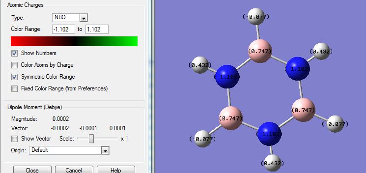
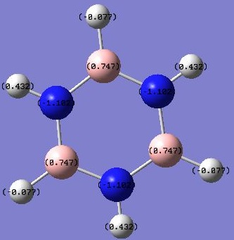
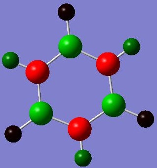
The NBO analysis showed distribution of charges on the atoms and images were captured and posted:
Showing coloured charges: (red means negative, green means positive, range = 1.1 to -1.1)
SHowing numbered charges:
As expected from the electronegativities of the atoms: (N 3.0, H 2.1, B 2.0) Charges on the atoms: N(-1.1); H(-0.077 next to B, 0.432 next to N); B(0.747). This agrees with the prediction based on relative electronegativities. The H atoms next to N atoms have their electron densities pulled away from the H atoms therefore having a more positive charge; the H atoms next to B atoms pull electron densities towards the H atoms and are more negative.
Comparison of Results of Benzene, Boratabenzene, Pyridinium and Borazine
This trend of molecules are summarised and compared in terms of the charge distribution and the resulting MO's.
Comparison of Charge Distribution
A brief summary and comparison of the charge distribution of the bezene, boratabenzene, pyridinium and borazine molecules calculated were tabulated below:
From this table we can see that, N atoms are the most negatively charged since they have a highest negativity of 3.0 and pulls electrons towards their atoms. C has electronegativity of 2.5 and pulls electrons less strongly, followed by H 2.1 and B 2.0. B atoms are the most positively charged as electron density is being pulled away from them by more electronegative H, C, N atoms.
Benzene has a uniform charge distribution, with C's having the same -0.239 and H's having +0.239, due to C having an electronegativity of 2.5 and H 2.1, so C atoms pull electron density from H, giving rise to the charge. The benzene molecule is symmetric and therefore the charges are distributed evenly.
Boratabenzene has one C substituted by a less electronegative B atom (B2.0 vs H 2.1, C 2.5). Being even less electronegative than H, the B atom donates electron density to H and C atoms next to it, giving rise to an uneven distribution of charge density. The ortho-C's are more negatively charged since the donating effect from B is the most significant. The second most negatively charged C is the para-C instead of the meta-C, due to the para-directing effect, i.e. this electron donating effect/ withdrawing effect is always strongest on the ortho- atom, then the para-atom (instead of the normally expected meta-atoms). The geometry is a greater effect than the "apparent distance" of two bonds for meta- being closer to the heteroatom. The H's next to the differently charged C atoms are affected accordingly - generally the more negatively charged the C/B is, the more positvely charged the neighbouring H atom will be.
Pyridinium is affected in a similar manner, the only difference being that the hetero-atom substituting one of the C atoms is a more electronegative N (N 3.0, C 2.5, H 2.1). As explained, the ortho-C is the most significantly affected by the electron-withdrawing N, second most affected is the para-C (due to the para-directing-effect), the least affected are the meta-C's. The H atoms are affected accordingly, in a similar manner explained for boratabenzene.
The borazine molecule comprises alternating N and B atoms, which are more (N 3.0) and less (B 2.0) electronegative than terminal H atoms (H 2.1). The charges on all N atoms -1.102 are identical and those on B 0.747 are also identical, so as for the neighbouring H-atoms (N-H 0.432) and (B-H -0.077) due to electron-withdrawal of N's and electron-donation of B's.
The charge distribution of these species can also be explained by invoking the theory of their resonance forms. The negatively charged atoms are atoms where electron density rests on in resonance forms. Resonance is a common observation on aromatic molecules because it provides extra stabilisation.
Comparison of MO's
The MO's computed were also summarised and compared between the four analogues and tabulated below:
Discussion
MO's chosen for the analysis are #7, the totally bonding sigma AO generated MO; #17, the totally bonding pi AO generated MO; and #20, the pi bonding MO of the second lowest energy, having two nodes. The MO's for the isoelectronic analogues generally have the same shapes and agree perfectly to the LCAO-predicted models.
By comparing the three chosen MO's a trend of MO energies could be obtained. Pyridinium has the lowest energy MO's, being the most stable; borazine has the second lowest energy MO's; followed by benzene; and boratabenzene has the highest energy MO's of all. This can be explained by the number of electronegative atoms present in the analogues. Taking benzene as a reference point, the pyridinium molecule has one N instead of a C, which has a higher electronegativity. The AO's contributing to LCAO are CN bonds - since CN bonds are stronger than CC bonds, and have a lower (more negative) energy, the MO's formed are lower in energy, too. A similar argument can be applied to boratabenzene, in which case an electropositive B is substituted, which has higher energy orbitals (B is electropositive and the orbitals are higher in energy in an MO diagram). The analogue therefore has the highest energy among the four derivative. As for borazine, there are three electronegative N atoms, but another three electropositive B atoms substituted the original C atoms. The level of electrogenativity of the resulting borazine MO's can be predicted by considering the relative increase of electronegativity of the molecule due to substitution by three N (N 3.0 vs C 2.5), and the relative decrease of electronegativity of the molecule due to substitution by three electropositive B (B 2.0 vs C 2.5). From this hypothesis we can make the prediction that the increase and decrease in electronegativity will pretty much average out, leading to an energy similar to that of benzene MO's.
It can also be seen from the coloured MO's that electron density prefers to stay on the electronegative N atoms, instead of the less negative B atoms, most easily observed from the borazine orbital #7, where the electron density adopts a triangular shape basing on the N atoms and avoiding the B atoms. The electron cloud in boratabenzene orbital #7 also prefers to avoid the electropositive B and likes resting on the more electronegative C's instead. This effect is less obvious in orbitals #17 and #20 due to the less strong interaction of the orbitals, since they are formed by the interaction of pi AO's which are higher in energy intrinsically.
Another summary table is made for a clearer comparison of the MO energies:
| Benzene | Boratabenzene | Pyridinium | Borazine | Difference in energy levels of MO's | |
|---|---|---|---|---|---|
| Orbital 7 (In order of increasingly positive orbital energy) | 3 | 4 | 1 | 2 | large energy difference between analogues |
| Orbital 17 (In order of increasingly positive orbital energy) | 2 (very close to energy of borazine MO) | 4 | 1 | 3 (very close to energy of benzene MO) | medium energy difference between analogues |
| Orbital 20 (In order of increasingly positive orbital energy) | 3 | 4 | 1 | 2 | small energy difference between analogues |
For the same specified MO, the difference in energy between the same MO for the analogues are also different, this can be explained by the nature of the MO's itself. For Orbital #7, the difference in energy between the derivatives is large (most negative -1.00398 v.s. most positive -0.9070, a difference of about 0.1 a.u.), while this difference in energy is small for orbital #20, that for orbital #17 lies between the two sets of values. This can be rationalised by thinking about the MO's themselves. For instance, for orbital #7, it is a totally bonding combination of the sigma orbitals. Sigma orbitals are lower in energy than pi orbitals, and this totally bonding combination leads to a great stabilisation. Therefore, the AO's contributing to this interaction combine to form the #7 MO, and since the stabilisation is large, the difference in energy of the corresponding AO's between the four species are amplified, giving a large difference in energy in the product MO's. Orbital #17 is the totally bonding combination of the pi orbitals, which also result in a stabilisation but the amount is smaller due to the originally higher energy nature of the contributing pi AO's. This gives rise to the amplification of the difference in energy of the contributing AO's as well but the effect is smaller. For orbital #20, the MO is formed by a less bonding combination of the AO's, this is reflected by the small energy difference (most negative -0.38968 a.u. v.s. least negative -0.36669 a.u., having a difference of about 0.02 a.u. as opposed to the much larger 0.1 a.u. in the case of orbital #7).
References
[1] J. Glaser, G. Johansson. Acta Chemica Scandinavica, 1982, 36a, Pp. 125-135.

