Rep:Mod:explosivesheep

Section 1: Introduction to the Ising Model

Minimum Energy Configuration

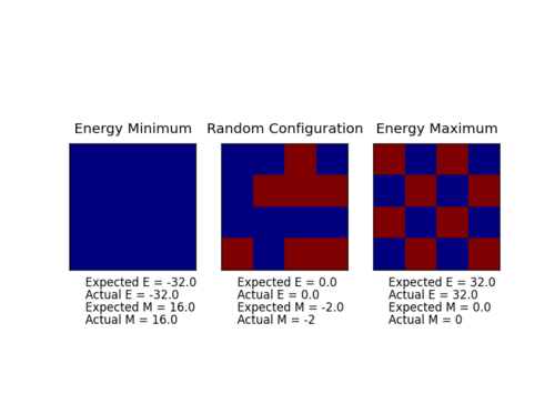
Energy of a lattice is minimised when all spins are parallel and all spin pair have the same interaction energy. When the spin interaction term become a constant, we can consider the number of interactions per spin as instructed by the summations. The boundary conditions mean that all spins have the same amount of interactions.

$\begin{aligned} E_{0} & = - \frac{1}{2} J \sum_{i}^{N} \sum_{j \in n e i g h b o r s (i)}^{} S_{i} S_{j} \\ = - \frac{1}{2} J \sum_{i}^{N} \sum_{j \in n e i g h b o r s (i)}^{} \underset{parallel spins}{\underset{⏟}{(+ 1)}} \\ = - \frac{1}{2} J \sum_{i}^{N} \underset{has 2 neighbors in each dimension}{\underset{⏟}{(2 D)}} \times (+ 1) \\ E_{0} & = - D N J \end{aligned}$

The minimum energy configuration has two microstates, since s_is_j = +1</math> for both when both spins are +1 and -1. The multiplicity of this state is 2.

$\begin{aligned} S_{0} & = k_{B} \ln W \\ = k_{B} \ln (2) \\ S_{0} & = 9.57 \times 1 0^{- 24} J K^{- 1} \end{aligned}$

Spin Flip

To move to a higher energy state, one of the spins change direction. The change in energy that results from this one spin flip is the above formula with the 1/2 factor removed since we are only considering one spin. The interaction energy between a pair of spins is changed from +1 to -1, and the change in the S_iS_j term is therefore -2.

$\begin{aligned} Δ E_{f l i p} & = - J \times \underset{has 2 neighbours in each dimension}{\underset{⏟}{(2 D)}} \times \underset{Δ s_{i} s_{j}}{\underset{⏟}{(- 2)}} \\ = 4 D J \end{aligned}$

The total energy after the spin flip is:

$\begin{aligned} E^{'} & = E_{0} + Δ E \\ = - D N + 4 D J \\ For a 10x10x10 (N=1000, D=3) lattice: \\ E^{'} & = - 2988 J \end{aligned}$

Since the spin flip can occur in all of the 10³ sites and in 2 directions(-1 to +1 and +1 to -1), there are $2 \times 1 0^{3}$ microstates.

$\begin{aligned} Entropy of the system after spin flip, S & = k_{B} \ln (2 \times 1 0^{3}) \\ And the change in entropy, Δ S & = k_{B} \ln (2 \times 1 0^{3}) - k_{B} \ln (2) \\ Δ S & = + 6.91 k_{B} = + 9.53 \times 1 0^{- 23} J K^{- 1} \end{aligned}$

Magnetisation

Magnetisation of a lattice is simply the sum of all spins inside the lattice.

$M = \sum_{i}^{N} s_{i}$

For the lattices in Figure 1, the magnetisations are:

$\begin{aligned} M_{2 D} & = 3 (+ 1) + 2 (- 1) & = + 1 \\ M_{3 D} & = 13 (+ 1) + 12 (- 1) & = + 1 \end{aligned}$

At absolute zero, the system only occupies its ground state with the parallel spins. As I mentioned above, this system has two microstates with either all +1 spins or -1 spins in each cell.

$M = \sum_{i}^{N} \pm 1 = \pm 1000 for N=1000.$

Section 2: Calculating Energy and Magnetisation

I completed the IsingLattice.energy() and .Magnetisation() functions, and the code can be found here with comments. The energy calculated uses the reduced term in units of <math>k_B</math>, which is the assumed unit from now on. The ILcheck.py script confirmed that these functions returned the correct values.

Section 3: Introduction to Monte Carlo Simulation

There are two possible states for each cell. For a 100-cell system,

$number of configurations = 2^{100} = 1.27 \times 1 0^{30}$ .

The time to evaluate all of these configurations with a rate of one million per second is:

$T i m e = \frac{2^{100}}{1 0^{9}} = 1.27 \times 1 0^{21} seconds = 4.02 \times 1 0^{10} millennia !$

Fortunately Monte Carlo simulation is much quicker and the code for my implementation can be found here with comments as self.montecarlostep().

The Curie temperature, T_C, is the phase transition temperature below which the system becomes ferromagnetic. In ferromagnetic systems we expect to see a spontaneous non-zero magnetisation ( $< M > \neq 0$ ).

[File:Jc Finalframe 1.png|thumb|Final output of ILanim.py]]

The ILanim.py script reached equilibrium below the Curie temperature after 300 steps , where magnetisation is non-zero and energy equals -DNJ.

The self.statistics function gave the following values:

$\begin{aligned} < E > & = - 1.438729348722 & < E^{2} > & = 2.30823794438 \\ < M > & = - 0.667910193792 & < M^{2} > & = 0.54006295332 \end{aligned}$

Section 4: Accelerating the Code

self.energy() and self.magnetisation() functions are optimised using numpy functions. The full code can be found here with comments.

Performance of the Simulation

Time to perform each Monte Carlo step was improved.

	Before Acceleration	After Acceleration
Time To Perform 2000 Steps (seconds)	9.31648	0.329255
	9.31847	0.354413
	9.33162	0.345731
	9.31753	0.350458
	9.33174	0.337710
	9.31693	0.340441
Std. Error	0.00303186	0.00372735
Average (seconds)	9.32213 ± 0.00030	0.343001 ± 0.003727

The changes made a 4.5 s improvement on average per 1000 Monte Carlo cycles, which becomes significant considering the number of cycles needed to simulate the equilibrium state of a system. The energy calculations were taxing performance because it ran 2 loops on the array of lattices. Simple reordering and multiplication of lattices enables much faster computations.

Steps To Reach Equilibrium

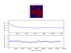
Because simulation at around Curie temperature will be required, I ran simulations around the theoretical Curie temperature (T = 2.69 ^[1]), at which the system is metastable, in addition to the stable T = 1.0 simulation specified in the given ILfinalframe.py script. Equilibrium around the Curie temperature is not so easy to reach and always required higher number of steps to reach equilibrium.

	7x7 at T=1.00	32x32 at T=2.69
Steps Needed To Reach Equilibrium	440	1830
	320	1250
	390	1930
	480	1180
	650	1390
	200	1260
Std. Error	62.16	133.34
Average	413 ± 62	1475 ± 133

Here I found out that there are some variation in the steps required. In later experiments, I will take the variation (~0.13 steps per spin) into account when devising the cutoff number. I also considered that temperature was not the only factor that affects the number of cycles required to reach equilibrium. I modified the ILfinalframescript producing a graph to compare the number of steps needed for other system sizes at different temperatures.

Notice that roughly 25000 steps was required for 32x32 at 1.0K to reach equilibrium, with the graph remaining asymptotic for many cycles. This represents a requirement of roughly 24.4 steps per spin. But setting a global cutoff to 25000 would be quite wasteful in terms of usable data points for the smaller lattices, and I compromised by scaling this cutoff limit with the number of spins:

	def __init__(self, n_rows, n_cols):
		......
		self.equilibrium_cycle = n_rows * n_cols * 25
		#set the equilibrium to scale according to the number of spins

The per-spin cutoff number is slightly raised from 24.4 due to the variations in this number which I investigated earlier. This change was made to IsingLattice.py for all the tasks below.

Effect of Temperature

I needed a large number of data points to gain an insight into the temperature effects on these thermodynamic parameters. The original ILtemperaturerange.py file stated a runtime of 150000. As a result of the cutoff scaling, the worst case scenario was omitting 25600 steps required for 32x32, with the cutoff point representing 1.7% of all data. I thought this gave a reasonably large proportion of samples so I have kept the original value. I am aware that I could have scaled the runtime as well according to the number of spins, but this would involve changing all of the given scripts and I was unsure if I was allowed to do so.

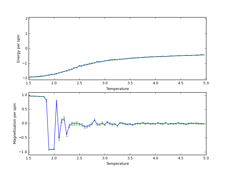
The plot below shows the energy and magnetisation at different temperatures with different systems, ranging from 1.5 to 5.0 K in 0.15 K increments. This was simulated by this script, and the cutoff implementation is in the IsingLattice class.

The error bars are very small with the exception of the data points around the Curie temperature. This was expected and already taken into account in the cutoff point. Even at around the Curie temperature, the error was quite acceptable at just less than 0.1K.

Section 6: The Effect of System Size

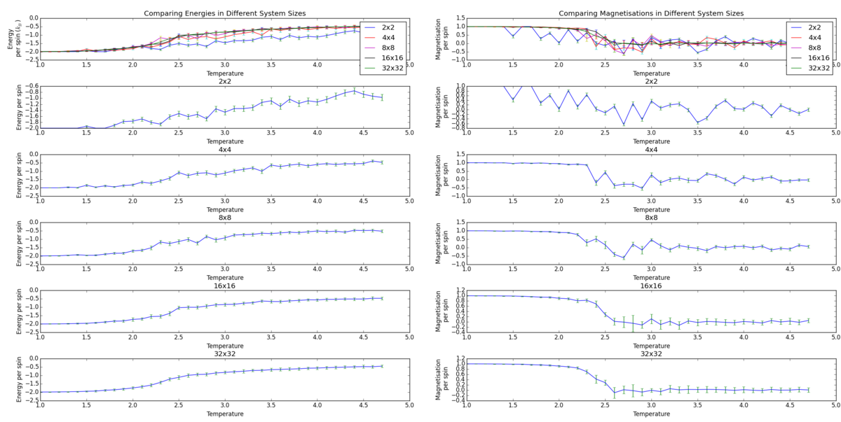
A script was written to loop through 2x2, 4x4, 8x8, 16x16 and 32x32 lattice environments and saving them in .dat files with the numpy savetxt function. Another script was written to load these texts and plot the following graph.

The output plot shows that the maximum asymptote for energy per spin increases for larger system sizes. The Curie temperatures, where magnetisation dramatically decreases, become progressively higher for larger system sizes. We can see that the 2x2 system is especially poor with the phase transition occurring over a range of almost 1.0 K. The decrease in magnetisation is also sharper for a large system size and I would expect a real-world plot to illustrate a sharp phase transition like in the larger system sizes. The error bars show a considerable amount of variance of energy and magnetisation at the phase transition region.

Section 7: Determining The Heat Capacity

The Relationship Between Heat Capacity And Energies

Heat capacity can shown to relate to the variance of energy.

Calculating Heat Capacities

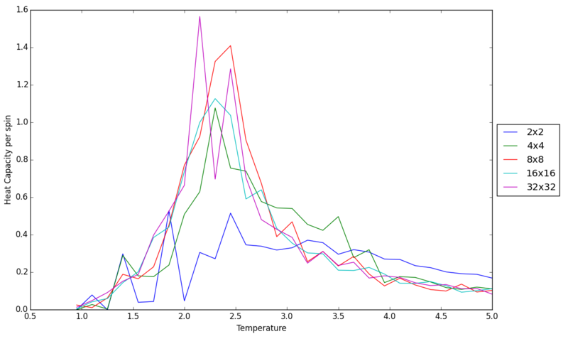
With the statistics data saved in the previous section, I wrote a script to calculate and plot heat capacities with respect to temperature for different system sizes. The temperatures range from 1.0 to 5.0K in 0.15K increments.

As you can see, the graphs are not continuous, especially around the Curie temperautre. Overall, the peaks approaches infinity and the Curie temperature decreases as we increase the system size. This behavior in the variance of accessible energy levels was expected as we have a larger canonical ensemble.

Comparing Simulation Data

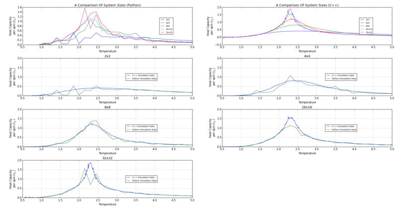
I used matplotlib to compare simulation data that I generated in python and data given in the script.

The C++ agrees with Python simulation data in the general shape. Because of the precision in the C++ data, the graphs look more continuous and easier to model. The fast calculations enabled by C++ allows more data points for analysis of the Ising model. A lower increment is needed to investigate the precise location of the Curie temperature where the heat capacity peaks. Another improvement would be to dramatically increase the runtime for larger lattice sizes as my simulation struggled to find the peak of the heat capacity, suggesting that the data does not have enough variance.

Section 8: Locating the Curie Temperature

The script for this section as a whole can be found here. The coding for each task follows the previous task because some data are continuously in use, and I thought it would be nice to get all the fits on one plot.

Polynomial Fits Over Whole Range

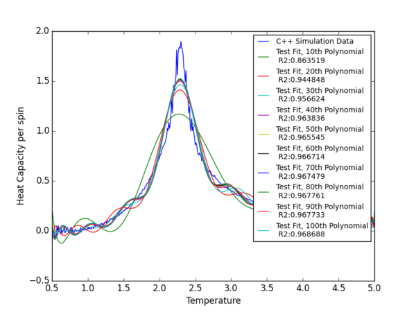
Initially I used various polynomial fits of different powers to test out the sensitivity of the fit accuracy with respect to the degree of polynomials. What I found was the fit improved as we increase the degree, measured by the coefficient of determination. But this improvement slowed at the 50th power of T, and any bigger powers of T had a very small contribution to the fitted curve and gave diminishing returns on improvements to coefficient of determination. To illustrate this, I plotted various polynomial fits onto the most complex set of data, the 64x64 lattice. The code used to plot the following graph can be found here.

I am not surprised with the poor fits even with very high powers of polynomials. The heat capacity function is almost discontinuous and theoretically approaches infinity at the transition temperature. I think that R² = 0.96 does represent an accurate fit with this imperfect polynomial model and gives a good estimate of the peak. Hence I applied the 50th order polyfit to all system sizes. I used a numpy function to find a positive root for the derivative of the polynomial fit. I also calculated the coefficient of determination for the fit.

System Size	Equation From Polynomial Fit (omitting coefficients that are less than 0.1)	Coefficient of Determination	Curie Temperature	Heat Capacity per spin at peak (k_B)
2x2	$\begin{aligned} - 0.1 x^{12} + 3.3 x^{10} - 1.9 x^{9} - 66.0 x^{8} + 325.2 x^{7} \\ - 804.3 x^{6} + 1237.2 x^{5} - 1249.9 x^{4} + 830.0 x^{3} \\ - 348.3 x^{2} + 83.5 x^{1} - 8.7 \end{aligned}$	0.998397	2.520189	0.414208
4x4	$\begin{aligned} - 0.2 x^{12} - 2.3 x^{11} + 7.0 x^{10} + 48.2 x^{9} - 391.1 x^{8} \\ + 1321.0 x^{7} - 2707.1 x^{6} + 3682.1 x^{5} - 3402.9 x^{4} \\ + 2114.1 x^{3} - 844.3 x^{2} + 195.5 x^{1} - 19.9 \end{aligned}$	0.999604	2.443764	0.815667
8x8	$\begin{aligned} 0.1 x^{15} - 0.2 x^{14} - 3.4 x^{13} + 0.2 x^{12} + 89.3 x^{11} \\ - 97.0 x^{10} - 2051.2 x^{9} + 12113.6 x^{8} - 35353.7 x^{7} \\ + 65225.6 x^{6} - 81432.5 x^{5} + 69924.6 x^{4} - 40717.0 x^{3} \\ + 15345.7 x^{2} - 3371.1 x^{1} + 327 \end{aligned}$	0.998141	2.35945	1.185714
16x16	$\begin{aligned} 0.5 x^{15} - 0.8 x^{14} - 14.7 x^{13} + 1.3 x^{12} + 379.7 x^{11} \\ - 424.0 x^{10} - 8654.1 x^{9} + 51314.7 x^{8} - 150052.4 x^{7} \\ + 277294.5 x^{6} - 346768.2 x^{5} + 298277.9 x^{4} \\ - 174002.2 x^{3} + 65704.9 x^{2} - 14463.2 x^{1} + 1406.1 \end{aligned}$	0.989282	2.318224	1.43101
32x32	$\begin{aligned} 0.1 x^{16} + 0.9 x^{15} - 1.1 x^{14} - 24.5 x^{13} - 4.5 x^{12} \\ + 626.9 x^{11} - 563.4 x^{10} - 14485.4 x^{9} + 82935.6 x^{8} \\ - 238122.0 x^{7} + 434126.9 x^{6} - 536889.1 x^{5} \\ + 457433.7 x^{4} - 264631.7 x^{3} + 99191.6 x^{2} \\ - 21689.9 x^{1} + 2095.9 \end{aligned}$	0.965545	2.287563	1.508265

The polyfit has a good coefficient of determination for all sizes, but especially so for the lower system sizes. We can see a clear trend of decreasing Curie temperatures with larger lattice sizes. Heat capacity also become more discontinuous at peak and increase in value with larger lattice sizes.

Fitting At A Particular Range

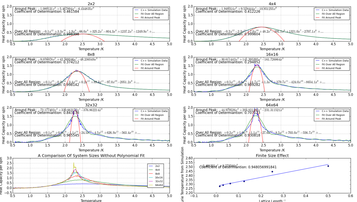
Since coefficient of determination was a good indicator of the accuracy of the fit, I have chosen this as a parameter for the range of particular data in the next polynomial fit. The algorithm for choosing the data points can be seen in the Python script. The small number of data point means that I do not have the liberty to choose a large degree of polynomial fit. The narrow range also me to choose a second-order polynomial for the fit, keeping analysis simple. If I had used a more complex polynomial, the presence of numerous maxima in such a small region could present problems for finding an actual maxima.

The particular region fit precisely represents the trend around the peaks in heat capacity except in the cases of small lattice systems. The coefficient of determination of this particular fit is calculated by comparing the fitted values with the actual data in the particular region only. I have used the peak obtained in this fit to calculate the Curie Temperatures.

System Size	1/L	Curie Temperature
2x2	0.5	2.510208
4x4	0.25	2.446616
8x8	0.125	2.334122
16x16	0.0625	2.309519
32x32	0.03125	2.290628
64x64	0.015625	2.261737

These data allowed me to plot Curie temperature v. 1/L to explore the linear relationship $T_{C, L} = A (\frac{1}{L}) + T_{C, \infty}$ . The plot with its linear fit can be seen on the bottom right of the multi-plot. The fit suggests that the Curie temperature, $T_{C, \infty} = 2.279586 \pm 0.118408$ in an infinite lattice (errors calculated from the coefficient of determination). The theoretical calculation for such a lattice is 2.269185^[1], within the lower bounds of my result.

Conclusion

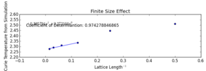
Although the simulation data agree with theoretical calculations, the theoretical result only lies on the very lower limit of my calculations. We have overestimated the y-intercept. It is evident from the infinite size effect plot that the small lattice size systems contribute to this inaccuracy. If only the larger 8x8, 16x16, 32x32 lattices are included, the y-intecept would be much lower. The inaccuracies of small lattice sizes also manifest in the lack of discontinuity at the Curie temperature and as a result, the fit over whole region had a better coefficient of determination than the fit over the particular region. It would be interesting to see if the whole-range fit would be more suitable for these small sizes. Even as models for energy and magnetisation, small systems do not represent the reality. These simulations lack the distinguished sudden drop of magnetisation at the transition temperature, which is in direct disagreement to experimental results.This was not unexpected since the Boltzmann distribution originates from the Stirling approximation of Boltzmann's entropy formula $S = k_{B} \ln W$ and is only valid for large numbers ( $N > 1 0^{2}$ ) of spins.

References

↑ ^1.0 ^1.1 L. Onsager, Phys. Rev, 1944, 65 (3-4), p.117, doi: 10.1103/PhysRev.65.117

[:0-1] 1.0 ^1.1 L. Onsager, Phys. Rev, 1944, 65 (3-4), p.117, doi: 10.1103/PhysRev.65.117

[1]