
Rep:Mod:emitretniw
Modelling using Molecular Mechanics
Rapid technological advances in the past two decades have caused similar developments in the area of computational chemistry. An ever growing field, it has expanded to such an extent that it is now not uncommon to find entire papers based on computationally derived data (the Journal of Computational Chemistry is dedicated to this field). The tools now accessible to chemists on through this platform, have allowed for versatile experiments to be conducted whereby theoretical data-sets can be generated - to serve as a comparison for those obtained experimentally.
This module will aim to demonstrate the power of some of these techniques - including
- optimisation of molecular structures using various methods (Allinger MM2[1]/MMFF94[2]/Mopac)
- visualisation of molecular orbitals
- simulation of 13C and 1H spectra from pre-optimised molecular geometries
All calculations performed will be submitted to the SCAN server to maximise time efficiency.
The Hydrogenation of Cyclopentadiene Dimer
Cyclopentadiene readily dimerises via a Diels-Alder π4s + π2s cycloaddition (Figure 2) which results in either the formation of the exo or endo dimer (Figure 1). The favoured conformation in this process is the endo-dimer, as confirmed in previous literature[3].
 |
 |
The MM2 method was performed on the two molecules to yield the table of energy contributions presented below:
| Parameter | Energy of exo-dimer(kcalmol-1) | Energy of endo-dimer(kcalmol-1) |
|---|---|---|
| Stretch | 1.2850 | 1.2509 |
| Bend | 20.5805 | 20.8477 |
| Stretch-Bend | -0.8381 | -0.8358 |
| Torsion | 7.6554 | 9.5109 |
| Non-1,4 VDW | -1.4173 | -1.5439 |
| 1,4 VDW | 4.2334 | 4.3201 |
| Dipole-Dipole | 0.3775 | 0.4476 |
| Total Energy | 31.8764 | 33.9975 |
Having been provided with the respective energy contributions of the respective exo and endo dimers, one can attempt to draw a conclusion on whether the cyclodimerisation is in fact kinetically or thermodynamically controlled. At first glance, one may take the lower energy of the exo-form as an indicator for increased stability relative to the endo-form. However, one knows – this is not the case.
The energy difference of 2.1211 kcal mol-1 can be primarily attributed to the increased torsional strain of the C-C-C-C bond (inclusive of the formed bond in dimerization) of the endo-form. This is perhaps best understood through visualisations (from same point-of-view) of the two molecules. As can be seen from the four highlighted carbon atoms, the C-C bonds in the exo-form (Figure 3) essentially adopts an antiperiplanar (app; 177.3°, 178.6°) conformation and that the endo-form (Figure 4) prefers the synclinal (sc; -45.8°, 51.2°) arrangement.
 |
 |
Thus, it can be said that the exo-form is the thermodynamically preferred product. In terms of steric considerations, its a.p.p. conformation is favoured over the gauche endo-form – due to lower destabilisation through Pauli repulsions between occupied C-H σ orbitals. The orbital overlap argument also stands for the a.p.p. form, as efficient σ-σ* overlap (E2 stabilisation) can be achieved in such a scenario.
In contrast, the kinetic product at standard conditions is the endo-dimer – formed in preference, in spite of lower thermodynamic stability. This can be primarily thought of in terms of the addition secondary overlap interactions available through the endo-dimer reaction pathway. [4]. HOMO-LUMO overlap between correctly aligned p-orbitals define this effect . [5]
At this stage, it is worth noting one of the potential limitations of the MM2 method – that transition state structures are not considered. For example, despite the endo-form being favoured under standard conditions, hypothetically, an equilibrium favouring the exo-form may be arrived at (upon increasing the temperature of the system). A lower activation energy, hence lower energy transition state for the exo-pathway.
Hydrogenation of the endo-dimer
The endo-dimer discussed previously can be subsequently be hydrogenated to afford two dihydro derivatives (3 and 4) depicted in Figure 1 (above).
As above, MM2 optimisations were performed on the two molecules, with the results summarised in the table below:
| Parameter | Energy of dihydro derivative 3(kcalmol-1) | Energy of dihydro derivative 4(kcalmol-1) |
|---|---|---|
| Stretch | 1.2777 | 1.0965 |
| Bend | 19.8587 | 14.5244 |
| Stretch-Bend | -0.8345 | -0.5494 |
| Torsion | 10.8110 | 12.4974 |
| Non-1,4 Van der Waals | -1.2227 | -1.0701 |
| 1,4 Van der Waals | 5.6328 | 4.5126 |
| Dipole/Dipole | 0.1621 | 0.1406 |
| Total Energy | 35.6850 | 31.1520 |
The large difference in “Bend” energies between the two dihydro derivatives can be traced back to the strain at the unhydrogenated carbon double bond in both structures. An sp2 carbon would usually prefer to adopt a 120° bond angle however this angle is 107.8° and 112.4° in structures 3 and 4 respectively. This confirms the thermodynamic preference for the formation of derivative 4. It is difficult to ascertain the kinetic product using purely the MM2 method.
The concept of atropisomerism arises due to hindered rotation about a single bond – leading to steric strain and generally undesirable interactions.
An example of this phenomena can be observed in the synthesis of taxol, in which compound A undergoes an Oxy-Cope Rearrangement[6] to yield atropisomers 1 and 2 (presented below in Figure 5). The crucial difference between two isomers is that the carbonyl group is aligned “down” in one and “up” in the other.

The relative stability of the two isomers can be investigated by optimising their geometries using the MM2 model (as previously) and MMFF94 model. Data generated is presented below:
| Parameter | Taxol atropisomer 1 (kcalmol-1) | Taxol atropisomer 2 (kcalmol-1) |
|---|---|---|
| Stretch | 2.7839 | 2.6216 |
| Bend | 16.5406 | 11.3402 |
| Stretch-Bend | 0.4299 | 0.3436 |
| Torsion | 18.2570 | 19.6657 |
| Non-1,4 VDW | -1.5569 | -2.1582 |
| 1,4 VDW | 13.1102 | 12.8723 |
| Dipole-Dipole | -1.7250 | -2.0022 |
| Total Energy (MM2) | 47.8397 | 42.6830 |
| Total Energy (MMFF94) | 70.5564 | 60.5517 |
From the MM2 force field calculations summarised in Table 3, it can be seen that the preferred, i.e. lowest energy and most stable, conformation is isomer 2. This stability has consequences for isomer 1, which would be expected to adopt the conformation of isomer under thermal equilibrium. The relative stability of isomer 2 is confirmed by the MMFF94 energy calculations.
The cyclohexane ring on both isomers, preferentially adopt a chair conformation – however these are mirror images of each other. The fact that the cyclohexane component is fused and essentially “locked” relative to the rest of the molecule, renders any interconversions between chair and twist-boat (via half-chair/boat) very difficult given the high thermodynamic barrier.
Hyperstable alkenes
The marked stability of the taxol intermediate can be related to the concept of hyperstability[7] relative to alkenes. With the alkene functional group located next to a bridgehead, one might assume increased reactivity as a result of the high bond strain. The idea of olefinic strain is central to this argument. It is essentially the difference in energy from the strain of the olefin compared with its alkane equivalent (hydrogenated). This value is positive for most compounds (olefin strain is at higher energy), except for hyperstable alkenes – where it is lower than in the respective alkane.
This notion of hyperstability can be tested by comparing the energy of atropisomer 2 (Table 3a) with that of its hydrogenated form. For clarity's sake, the two molecules under consideration are presented below in Figure 5b:

Both molecules were subject to MM2 and MMFF94 methods, as previously.
| Parameter | Hydrogenated derivative (kcalmol-1) | Taxol atropisomer 2 (kcalmol-1) |
|---|---|---|
| Stretch | 2.9240 | 2.6216 |
| Bend | 13.0747 | 11.3402 |
| Stretch-Bend | 0.6607 | 0.3436 |
| Torsion | 25.9344 | 19.6657 |
| Non-1,4 VDW | -1.7784 | -2.1582 |
| 1,4 VDW | 17.0524 | 12.8723 |
| Dipole-Dipole | -1.7342 | -2.0022 |
| Total Energy (MM2) | 56.1336 | 42.6830 |
| Total Energy (MMFF94) | 80.1639 | 60.5517 |
The energies calculated using both methods definitively conclude that the hydrogenated derivative is higher in energy with respect to is non-hydrogenated counterpart. Hydrogenation of the double bond in this instance, albeit slightly counter-intuitive, is unfavourable from a stability standpoint.
Modelling Using Semi-empirical Molecular Orbital Theory
Regioselective Addition of Dichlorocarbene
The aim of this section is to explore the effect of electronic interactions within a molecule on its geometry and reactivity. Structures will be optimised using a combination of MM2 and Mopac/PM6 methods. The [1+2] cycloaddition of 9-chloromethanonaphthalene (Compound A) with dichlorocarbene displays marked selectivity, to yield the syn regioisomer outlined below in Figure 7:

Compound A was initially optimised using MM2, before subsequently being subject to the Mopac/PM6 method.
An interesting observation can be made by superimposing the post MM2/Mopac optimised structures (Fig. 7b, below):
The Mopac/PM6 optimised structure is seen to lie below that of the MM2 structure. These differences help to shed light on the potential limitations of purely employing the MM2 method for optimisation.
Further examination of the HOMO of the optimised molecule (included below in Figure 8) revealed unexpected results. One would expect compound A to fall under the Cs point group, of which a prerequisite is having a σh plane of symmetry. This is clearly not the case when consulting Figure 8, which depicts asymmetry in the plane bisecting the C=C bond.

The Mopac/PM6 optimised structure was further optimised on the SCAN server, subjecting it to Gaussian parameters of DFT, B3LYP 6-31G (d,p). A population analysis was then conducted to further examine the molecular orbitals of compound 7.
The HOMO-1, HOMO, LUMO, LUMO+1, LUMO+2 orbital representations, as viewed through the GaussView interface, are presented below.
| Molecular orbital | HOMO-1 | HOMO | LUMO | LUMO+1 | LUMO+2 |
|---|---|---|---|---|---|
| Orbital representation |  |
 |
 |
 |
 |
The HOMO (Fig. 9) and LUMO (Fig. 10) orbitals will be considered first. One can see that electron density of HOMO is primarily concentrated on the syn-alkene. This equates to increased nucleophilicity of the C=C bond and therefore the greater likelihood of addition at that position. Regioselectivity of the dicarbene, in the aforementioned reaction (Figure 7) supports this idea (i.e. electron donation into LUMO of dicarbene). In contrast, the LUMO is susceptible to nucleophilic attack, as most of the electron density is located at the anti-alkene.
The LUMO+2 evidently depicts the σ* orbital of the C-Cl bond. Chlorine is especially electronegative, thus distorts the electron cloud away from carbon, leaving it electron deficient. Further examination of the HOMO-1 orbital reveals the ideal orientation of the C-Cl σ* orbital to overlap with the electron-rich pi cloud of the anti C=C bond. As electron donation occurs into an antibonding orbital, this serves to weaken the C-Cl bond. Moreover, the electron donation away from the anti C=C bond renders it less nucleophilic than its syn counterpart. This, once more, correlates with the observed regioselectivity– preference of electrophilic addition to the syn-alkene.
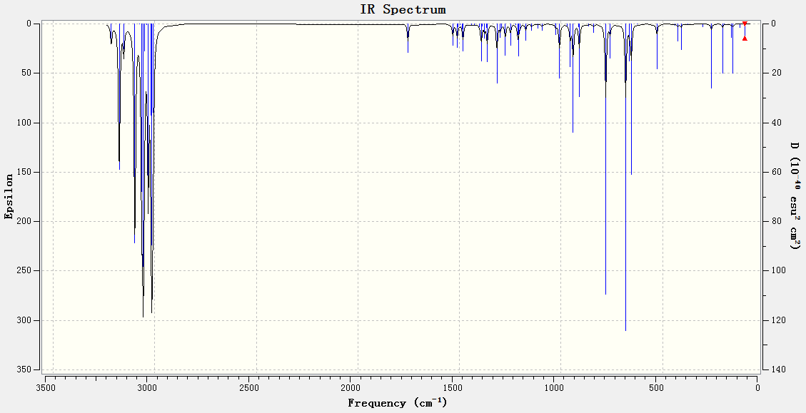
A further vibrational analysis was performed on the molecule to confirm the interaction of LUMO+2 and HOMO-1 orbitals. Comparisons were drawn to the monohydrated derivative (Figure 14, optimised in the same manner as compound A). The absence of the anti-alkene, will help to illustrate its electron donating effect to the σ* orbital.

The table below summarises the C=C (syn and anti) and C-Cl stretching frequencies obtained for both molecules:
| Bond | Original molecule | Monohydrated derivative |
|---|---|---|
| C-Cl | 770.91 | 779.93 |
| C=C (syn) | 1757.37 | 1753.76 |
| C=C (anti) | 1737.11 | - |
As expected, the C-Cl bond in the monohydrated derivative (IR spectrum) stretches at a higher (by roughly 9 cm-1) frequency than the original diene (IR spectrum). This confirms that without the presence of the anti-alkene (destabilising influence), electron donation into the antibonding σ* orbital is not possible – resulting in a stronger C-Cl bond.
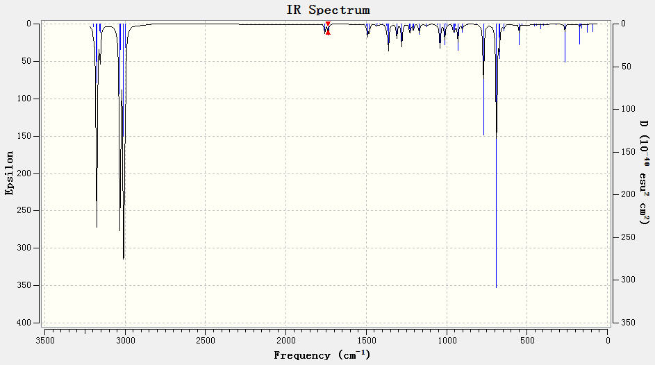
This assumption can be additionally tested by introducing a substituent to the anti-alkene of the original molecule. Hypothetically, an electron-withdrawing group such as –NO2 should serve as to decrease the electron density on the anti-alkene, and thus reduce the HOMO-1 – LUMO+2 interaction. Logically, this should result in a higher stretching frequency for the C-Cl bond (less destabilisation, stronger bond) than in the original diene. The opposite should be true for an electron-donating group such as –OMe, i.e. should result in a weaker C-Cl bond.
Two variants of the original diene (Fig. 15 & 16), were optimised as per the previous method, with the frequency analysis presented below in Table 6:
 |
 |
| Bond | -OMe substituent | -NO2 substituent |
|---|---|---|
| C-Cl | 765.13 | 771.55 |
| C=C (syn) | 1756.35 | 1758.06 |
| C=C (anti) | 1736.63 | 1738.91 |
The data clearly confirms the suggestions outlined above. It is perhaps worth adding that, with respect to the bond frequencies of in the original diene, the strength of the C=C (both syn and anti) mirrors the relative strength of the C-Cl bond.
Monosaccharide chemistry - a look at the mechanism for glycosidation
Glycosidation – forming a new glycosidic bond – occurs via an intermediate oxonium cation that results in the product being a mix of two different anomers. The influence of the –OAc group (adjacent to the anomeric carbon) on whether the alpha or beta anomer is formed is a prime example of the “neighbouring-group effect”. A standard glycosidation pathway is shown below in Figure 17 and outlines the formation of the two anomers. Note that R, in this instance, represents a methyl group (less cumbersome for data processing, i.e. no hydrogen bonding and no real steric issues, yet still acts as a protecting group).

It can be seen that the relative orientation of the –OAc substituent, with respect to the plane of the ring, is pivotal in determining the stereochemistry of the product. The beta-anomer arises through formation of the cationic oxonium intermediate on the bottom face of the ring. Nucleophilic attack subsequently proceeds via the top face at the anomeric carbon. The opposite is true for the mechanism relating to the alpha-anomer.
MM2 modelling in conjunction with Mopac/PM6 was used to investigate the participation of the acyl group during the formation of the oxonium ion. Through ChemBio 3D 12, the energies of structures A, B, C, D as well as their ring-flipped equivalents are presented in the table below:
| Parameter | A | A' | C | C' |
|---|---|---|---|---|
| Stretch | 2.6794 | 2.4007 | 1.9932 | 2.6876 |
| Bend | 11.4896 | 14.2083 | 13.0972 | 17.8431 |
| Stretch-Bend | 1.0331 | 0.9034 | 0.6844 | 0.8250 |
| Torsion | 1.4228 | 1.9841 | 7.4463 | 7.7920 |
| Non-1,4 VDW | 1.4526 | -0.4782 | -2.5289 | -2.7442 |
| 1,4 VDW | 18.4614 | 19.2566 | 17.7194 | 19.1464 |
| Charge-Dipole | -22.9197 | -24.8666 | -10.5186 | -3.2375 |
| Dipole-Dipole | 7.6971 | 11.2230 | -0.5345 | 0.3583 |
| Total Energy, MM2 | 21.3162 | 24.6313 | 27.3614 | 42.6707 |
| ΔH energy of formation, MOPAC/PM6 | -91.65214 | -60.92454 | -91.66021 | -67.47455 |
| Parameter | B | B' | D | D' |
|---|---|---|---|---|
| Stretch | 2.4380 | 2.4773 | 1.9110 | 2.5880 |
| Bend | 13.2763 | 13.5912 | 19.8603 | 16.4201 |
| Stretch-Bend | 1.0597 | 0.9636 | 0.6981 | 0.7207 |
| Torsion | 1.4187 | 0.8168 | 6.4506 | 6.9410 |
| Non-1,4 VDW | -2.2823 | -1.7618 | -3.3105 | -2.6487 |
| 1,4 VDW | 18.4902 | 18.3894 | 17.1876 | 19.4546 |
| Charge-Dipole | -6.9679 | -3.4048 | -4.5706 | -2.3815 |
| Dipole-Dipole | 6.1995 | 6.2416 | -1.8428 | -0.8298 |
| Total Energy, MM2 | 33.6321 | 37.3134 | 36.3836 | 40.2645 |
| ΔH energy of formation, MOPAC/PM6 | -89.63126 | -68.23402 | -88.72765 | -66.66096 |
| A (MM2/MOPAC) (eq, below) | A’ (MM2/MOPAC) (eq, above) | B (MM2/MOPAC) (ax, above) | B' (MM2/MOPAC) (ax, below) |
| C (MM2/MOPAC) (eq, below) | C’ (MM2/MOPAC) (eq, above) | D (MM2/MOPAC) (ax, above) | D’ (MM2/MOPAC) (ax, below) |
Note: Distinction between equatorial (eq) and axial (ax) relates to the orientation of the –OAc substituent relative to the hydrocarbon ring. “Above” and “below” relate to position of the –OAc group with respect to the plane of the 6-membered ring (for A, A’, B, B’) and 5 membered cationic intermediate with respect to the main ring (for C, C’, D, D’).
A comment can be made at this point, contrasting the MM2 and Mopac/PM6 methods. In this instance, MM2 has difficulty dealing with non-classical carbocations (oxonium cation) and conjugation in molecules. Yet the MM2 method is altogether competent, albeit for more classical hydrocarbon frameworks. In contrast, the Mopac/PM6 method is able to take account of the stabilising influence of the acetyl oxygen lone pair on the cationic intermediate. The “neighbouring-group” effect is thus successfully modelled and implies that the method is capable of “guessing” the formation of new bonds.
From the energies reported in Tables 7 and 8, it is clear that despite the differences discussed previously concerning the two models – they paint a similar picture.
When considering the MM2 method, the molecules as drawn in Figure 17 all show increased stability (lower energy) relative to its ring-flipped isomer. Taking into account the various contributions of this final energy term, it can be seen that there is marked difference in the value of the charge-dipole (energy) term. This observation ties in nicely with the previously discussed notion of MM2 not being able to properly recognise the oxonium cation, instead viewing the oxygen atom as a point charge. With this in mind, the value assigned to the charge-dipole energy is therefore directly correlated to the distance between the acetyl oxygen lone pair and the oxonium cation. One can infer that this distance is longer for the ring-flipped isomers (with the exception of A, possibly due to a miscalculation) than the original structures (as in Figure 17).
The Mopac/PM6 values for the heat of formation mirror the relative stabilities derived from the MM2 method (that A is more stable relative to A’ etc.). Interestingly, the pair of delta H values for A and C, as well as B and D are essentially the same (statement holds for ring flipped isomers). This observation supports the idea of the Mopac/PM6 model recognising potential bond formation between atoms.
It is perhaps also worth considering the trajectory at which the acetyl oxygen lone pair (nucleophilic HOMO) approaches the anomeric carbon (LUMO) of the oxonium cation. A comparison can then be made to the Burgi-Dunitz angle, at 107° – the optimum trajectory for nucleophilic attack at an sp2 hybridised atom. These values are presented for A and A’ pairs as well as B and B’ pairs below in Table 9:
| Molecule | Angle of attack (°) |
|---|---|
| A | 111.9 |
| A' | 128.0 |
| B | 105.1 |
| B' | 152.8 |
Mini Project
Modern computational techniques can additionally be employed to generate NMR spectra of various compounds. This technique will be applied to atropisomer 2, as depicted in Figure 4, from section 2.1 (taxol synthesis). The computed spectra will be compared with values provided in literature[8].
Atropisomer 2 was initially optimised using the MM2 method. Further calculation involved using the DFT (restricted B3LYP) method with 6-31G (d,p) basis set. To ensure the relevance of output spectral values with those in literature, the solvent system was specified. The CPCM solvation method was selected with benzene as solvent. Subsequently, an NMR calculation was performed using the mpw1pw91/6-31G(d,p) method with solvent method as before. Output was referenced with respect to TMS (mpw1pw91/benzene, GIAO)
The data generated for the 13C spectrum is presented below in Table 10, alongside a diagram of atropisomer complete with labelled carbon environments:
| Carbon # | Literature value | Experimental value | Difference |  |
| 8 | 211.49 | 210.72 | 0.77 | |
| 16 | 148.72 | 146.73 | 1.99 | |
| 17 | 120.90 | 118.57 | 2.33 | |
| 2 | 74.61 | 87.52 | -12.91 | |
| 19 | 60.53 | 60.56 | -0.03 | |
| 6 | 51.30 | 52.14 | -0.84 | |
| 10 | 50.94 | 51.45 | -0.51 | |
| 11 | 45.53 | 46.81 | -1.28 | |
| 3 | 43.28 | 45.12 | -1.84 | |
| 20 | 40.82 | 42.13 | -1.31 | |
| 21 | 38.73 | 40.92 | -2.19 | |
| 5 | 36.78 | 37.84 | -1.06 | |
| 9 | 35.47 | 35.98 | -0.51 | |
| 7 | 30.84 | 31.18 | -0.34 | |
| 18 | 30.00 | 29.55 | 0.45 | |
| 15 | 25.56 | 25.51 | 0.05 | |
| 13 | 25.35 | 23.78 | 1.57 | |
| 14 | 22.21 | 21.55 | 0.66 | |
| 4 | 21.39 | 21.43 | -0.04 | |
| 12 | 19.83 | 20.09 | -0.26 |
From looking at the difference between experimental (calculated) and literature values, it can be seen that essentially all values fall within a ±2.5ppm range. The notable outlier – carbon 2 – is highlighted in yellow. With a difference of almost 13ppm to the literature value, this discrepancy can be primarily attributed to the two adjacent sulphur atoms (part of a five-membered ring). Significant spin orbit interactions [9] may be experienced by carbon two as a result of the difference in nuclear mass between sulphur and carbon.
Secondly the proton NMR data (referenced to TMS, mpw1pw91/benzene, GIAO) calculated, was compared to literature values in Table X. Note that as specific chemical shifts were not provided for all literature values, individual proton environments were not assigned. A comment of “ok” was used (in place of the calculated difference) for when only a range was provided in literature – to signify falling within said ppm range.
| Literature value | Experimental value | Difference |
| 5.85 | 5.21 | 0.64 |
| 2.95 | 2.7 - 3 | ok |
| 2.95 | 2.7 - 3 | ok |
| 2.83 | 2.7 - 3 | ok |
| 2.83 | 2.7 - 3 | ok |
| 2.76 | 2.7 - 3 | ok |
| 2.67 | 2.7 - 3 | -0.03 |
| 2.59 | 2.35 - 2.7 | ok |
| 2.38 | 2.35 - 2.7 | ok |
| 2.38 | 2.35 - 2.7 | ok |
| 2.38 | 2.35 - 2.7 | ok |
| 2.21 | 1.7 - 2.2 | ok |
| 2.08 | 1.7 - 2.2 | ok |
| 2.08 | 1.7 - 2.2 | ok |
| 1.85 | 1.7 - 2.2 | ok |
| 1.85 | 1.7 - 2.2 | ok |
| 1.67 | 1.7 - 2.2 | -0.03 |
| 1.67 | 1.58 | 0.09 |
| 1.39 | 1.2 - 1.5 | ok |
| 1.39 | 1.2 - 1.5 | ok |
| 1.39 | 1.2 - 1.5 | ok |
| 1.39 | 1.10 | 0.29 |
| 1.17 | 1.10 | 0.07 |
| 1.17 | 1.10 | 0.07 |
| 1.05 | 1.07 | -0.02 |
| 1.05 | 1.07 | -0.02 |
| 0.83 | 1.07 | -0.24 |
| 0.83 | 1.03 | -0.20 |
| 0.74 | 1.03 | -0.29 |
| 0.47 | 1.03 | -0.56 |
In general, most of the data falls within ±0.30ppm of the literature value (range) –showing strong correlation between datasets. Chemical shift values at extreme ends of the spectrum (lit.: 5.85ppm, 0.47ppm) were found to differ significantly from calculated values (circa 0.60ppm).
Isomeric precursors for the synthesis of a bridgehead, “foiled carbene” [10]
Introduction
The concept of “foiled carbenes” was initially uncovered in the late 1960s by Gleiter and Hoffmann[11]. It was defined by the presence of a stereoelectronic interaction resulting from the presence of a carbene and olefin moiety[12] [13], within the same ring system. The vacant LUMO (p-orbital) on the bridgehead carbon interacts with the HOMO (double bond pi orbital). Differing from the conformation adopted by a “classical” bridgehead carbene, in a foiled carbene, the “divalent carbon bends toward the double bond”. This is illustrated in the diagram below:

Two isomeric oxadiazoline precursors - generated in the preparation of bicyclo[3.2.1]oct-6-en-8-ylidene (a classic example of a foiled carbene) will be subsequently examined in greater detail. The two isomers (4a and 4b) are presented below in figure 20:
 | ||||||
| 4a | 4b |
It can be seen that the only difference between the stereoisomers is the orientation of the five-membered ring at the bridgehead carbon. In each instance, the ring is locked in position relative to the rest of the molecule – preventing conformational interconversion between molecules 4a and 4b.
In molecule 4a, it is an oxygen atom that is potentially in a position to interact with the C=C double bond, whereas in 4b, this role is fulfilled by a nitrogen atom (N=N double bond). These interactions will be considered in greater detail in due course.
The formation of the two isomers from the respective bridgehead ketone is detailed mechanistically in Figure 21. Initial treatment with acetyl hydrazide in followed by oxidation with phenyliodinium diacetate. This reaction pathway is well documented in previous literature[14]

From the above mechanism, one will be able to grasp that the ultimate product formed (whether it be 4a or 4b) is dependent on direction the phenyliodinium diacetate attack - as illustrated below:

An important point worth noting is that molecule 4a is preferentially formed (with respect to 4b) in a 7:4 ratio. This notable bias towards 4a will hopefully be confirmed in the following energy analysis.
Structure optimisation
Molecules 4a and 4b were subject to the MM2 method, followed by MMFF94 and Mopac/PM6 optimisations. The output data is presented in Table X:
| Parameter | 4a | 4b | Difference |
| Stretch | 1.7566 | 1.7341 | 0.0225 |
| Bend | 13.8395 | 13.4681 | 0.3714 |
| Stretch-Bend | 0.133 | 0.1374 | -0.0044 |
| Torsion | 0.6382 | 2.14 | -1.5018 |
| Non-1,4 VDW | -3.3711 | -3.9881 | 0.617 |
| 1,4 VDW | 11.075 | 11.6028 | -0.5278 |
| Dipole/Dipole | 10.449 | 10.2675 | 0.1815 |
| MM2 - Total Energy | 34.5203 kcal/mol | 35.3619 kcal/mol | |
| MMFF94 - Final Energy | 52.226 kcal/mol | 52.8123 kcal/mol | |
| Mopac/PM6 - Heat of Formation | -34.50487 Kcal/Mol | -33.41238 Kcal/Mol |
With 4a preferentially formed, one would thus expect the MM2 and MMFF94 energies of 4a to be lower than 4b. This is indeed the case – supporting the additional stability of 4a. The value obtained for the heat of formation from the Mopac/PM6 method further backs up the view (delta H is more exothermic for 4a).
In terms of the difference between parameters contributing to the overall MM2 energy, the value for the torsional energy of 4b is almost 3.5 times that of 4a. This suggests the possibility of 4b adopting a more “foiled” conformation, thus resulting in greater steric strain.
| 4a (MM2/MMFF94/MOPAC) | 4b (MM2/MMFF94/MOPAC) |
Population analysis of frontier orbitals
The stability of both isomers was then considered from an MO standpoint by performing a population analysis. Prior to this calculation, 4a and 4b structures from the previous minimisations were further optimised using a DFT method (B3LYP), 6-31G(d,p) basis set. Molecular orbitals from HOMO-1 to LUMO+2 are presented below in Tables Xa and Xb. For further clarity, two separate points of view are offered for each visualisation.
| Molecular orbital | HOMO-1 | HOMO | LUMO | LUMO+1 | LUMO+2 |
|---|---|---|---|---|---|
| Side-view |  |
 |
 |
 |
 |
| View across C=C |  |
 |
 |
 |
 |
| Molecular orbital | HOMO-1 | HOMO | LUMO | LUMO+1 | LUMO+2 |
|---|---|---|---|---|---|
| Side-view |  |
 |
 |
 |
 |
| View across C=C |  |
 |
 |
 |
 |
From comparing the HOMOs of 4a and 4b, one will notice major differences. As the highest occupied bonding molecular orbital, any antibonding interactions between filled orbitals will serve as to destabilise the molecule. In 4b, the bonding C=C π orbital is correctly oriented to interact with the antibonding N=N π* orbital – therefore resulting in an unfavourable electronic situation. As the two nitrogen atoms are on the other side of the C=C double bond in 4a, this destabilising effect is absent. Moreover, the number of size of the bonding MOs in 4a are significantly larger than in 4b. An example is the consecutive interaction between σ bonding orbitals on six out of the seven carbon atoms on the C=C containing ring framework. The electron-rich double bond in both structures renders it markedly susceptible to electrophilic attack.
The concept of greater bonding interactions between orbitals is present also when comparing the HOMO-1 MOs. One will observe the interaction between bonding C=C π orbital and the bonding overlap of C-O p orbitals. This sort of significant delocalisation is not made possible in 4b, where the antibonding N=N π* orbital means that electron density can only be delocalised onto one of the nitrogens.
There are no major differences between LUMO to LUMO+2 orbitals of the two compounds. A point can still be made about the absence of any MOs from the C=C double bond (LUMO) and the N=N (LUMO+1) for molecule 4b. This suggests that 4b is not as reactive through the double bond as 4a.
NMR analysis
Spectral differences between 4a and 4b from literature data
As demonstrated in section 2.1, NMR analysis can prove conclusive in differentiating between two isomers. The 13C and 1H NMR values from literature will be compared with those calculated.
To begin with, it is perhaps worth noting the major differences in the spectra of the two compounds. Data from literature is tabulated below for comparison’s sake.
| 4a | 4b | Difference |
| 131.33 | 133.10 | -1.77 |
| 131.29 | 131.80 | -0.51 |
| 131.27 | 131.40 | -0.13 |
| 130.90 | 131.10 | -0.20 |
| 51.10 | 50.40 | 0.70 |
| 50.60 | 45.40 | 5.20 |
| 49.70 | 44.50 | 5.20 |
| 24.00 | 24.10 | -0.10 |
| 23.90 | 21.50 | 2.40 |
| 23.80 | 21.10 | 2.70 |
| 17.50 | 16.80 | 0.70 |
It can be seen that 4a has three peaks at around 50.00ppm, whereas only one is present in 4b (other two occur at around 45.00ppm). Aside from this major difference, all other peak pairs lie within the range attributed to reasonable experimental error.
The same data is presented for the proton NMR:
| 4a | 4b |
| 6.03 (m, 2H) | 6.15 (m, 2H) |
| 3.09 (s, 3H) | 3.10 (s, 3H) |
| 2.72 (m, 1H) | |
| 2.50 (m, 1H) | 2.45 (m, 1H) |
| 2.38 (m, 1H) | |
| 2.18 (m, 1H) | 2.18 (m, 1H) |
| 1.74 (m, 2H) | 1.8-1.6 (m, 3H) |
| 1.63 (s, 3H) | 1.67 (s, 3H) |
| 1.56 (m, 2H) | 1.5-1.4 (m, 3H) |
One will notice that there are two peaks (2.38 and 2.72ppm respectively) present in the proton spectrum of 4a which are not observed in that 4b. This should serve as a simple differentiating factor for the two compounds.
Simulation of 13C NMR spectra
Optimised molecules from the initial minimisations were carried forward to this stage. Further optimisation involved using the DFT (restricted B3LYP) method with 6-31G (d,p) basis set. The CPCM solvation method was employed, with chloroform as solvent. Subsequently, an NMR calculation was performed using the mpw1pw91/6-31G(d,p) method with solvent method as before. Output was referenced with respect to TMS (mpw1pw91/CDCl3 6-31G(d,p), GIAO)
Results for molecule 4a relative to literature values are presented below in Table X along with a diagram with labelled carbon environments.
| Carbon # | Literature value | Experimental value | Difference |  |
| 8 | 131.33 | 131.16 | -0.17 | |
| 1 | 131.29 | 128.70 | -2.59 | |
| 2 | 131.27 | 128.41 | -2.86 | |
| 9 | 130.90 | 127.61 | -3.29 | |
| 3 | 51.10 | 52.69 | 1.59 | |
| 7 | 50.60 | 50.35 | -0.25 | |
| 11 | 49.70 | 48.37 | -1.33 | |
| 6 | 24.00 | 23.72 | -0.28 | |
| 4 | 23.90 | 22.78 | -1.12 | |
| 10 | 23.80 | 17.82 | -5.98 | |
| 5 | 17.50 | 17.73 | 0.23 |
The three peaks at around 50.00ppm (as mentioned previously) are all present, albeit with minor deviations of at most 1.60ppm. Carbons 9 and 10 differ from literature values significantly – 3.29 and 5.98ppm respectively. In essence, these two carbon environments are isolated from the rest of the carbon framework.
Similar values for molecule 4b are presented below in Table X:
| Carbon # | Literature value | Experimental value | Difference |  |
| 8 | 133.10 | 132.75 | -0.35 | |
| 9 | 131.80 | 129.33 | -2.47 | |
| 2 | 131.40 | 128.67 | -2.73 | |
| 1 | 131.10 | 128.30 | -2.80 | |
| 11 | 50.40 | 50.49 | 0.09 | |
| 3 | 45.40 | 46.79 | 1.39 | |
| 7 | 44.50 | 45.71 | 1.21 | |
| 4 | 24.10 | 21.27 | -2.83 | |
| 6 | 21.50 | 20.80 | -0.70 | |
| 10 | 21.10 | 17.28 | -3.82 | |
| 5 | 16.80 | 16.70 | -0.10 |
Almost all calculated values lie within a reasonable range of the theoretical values. The largest difference arises from carbon 10 (once more!) – at 3.82ppm. This suggests that in reality, the carbon is interacting with neighbouring atoms , therefore offsetting the chemical shift value. Additional investigations could be conducted using a different Gaussian method or basis set to better reflect the additional interactions experienced at carbon 10.
Simulation of 1H NMR data
In the same manner as for the 13C NMR, data from the 1H spectra of molecules 4a and 4b were obtained. As previously mentioned, the literature values were not entirely absolute (several ppm ranges given instead), thus gaps have been left in the comparison table below.
| 4a literature value | 4a calculated value | Multiplicity | 4b literature value | 4b calculated value | Multiplicity |
| 6.03 (m, 2H) | 6.48 | 1 | 6.15 (m, 2H) | 6.49 | 2 |
| 6.41 | 1 | 3.10 (s, 3H) | 3.83 | 1 | |
| 3.09 (s, 3H) | 3.50 | 3 | 3.70 | 1 | |
| 2.72 (m, 1H) | 2.64 | 2 | 3.43 | 1 | |
| 2.50 (m, 1H) | 2.48 | 1 | 2.45 (m, 1H) | 2.42 | 1 |
| 2.38 (m, 1H) | 2.16 | 1 | 2.32 | 1 | |
| 2.18 (m, 1H) | 2.09 | 1 | 2.18 (m, 1H) | 2.17 | 1 |
| 1.74 (m, 2H) | 1.93 | 2 | 1.8-1.6 (m, 3H) | 1.68 | 4 |
| 1.69 | 1 | 1.67 (s, 3H) | 1.30 | 3 | |
| 1.63 (s, 3H) | 1.61 | 1 | 1.5-1.4 (m, 3H) | 1.07 | 1 |
| 1.56 (m, 2H) | 1.46 | 1 | |||
| 1.12 | 1 |
From the proton NMR data calculated, the distinction between the two compounds is not as immediately obvious, relative to the 13C NMR data. The two singlets observed in literature at 2.38 and 2.72ppm are present in the calculated spectrum. However, that at 2.64ppm (lit: 2.72ppm) is a doublet. These two peaks are not seen in 4b, for which the only expected singlets between 2-3ppm occur at 2.17ppm (lit: 2.18ppm) and 2.42ppm (lit: 2.45ppm). It must be mentioned that the singlet at 2.32ppm in the calculated spectrum of 4b is somewhat anomalous based on literature values.
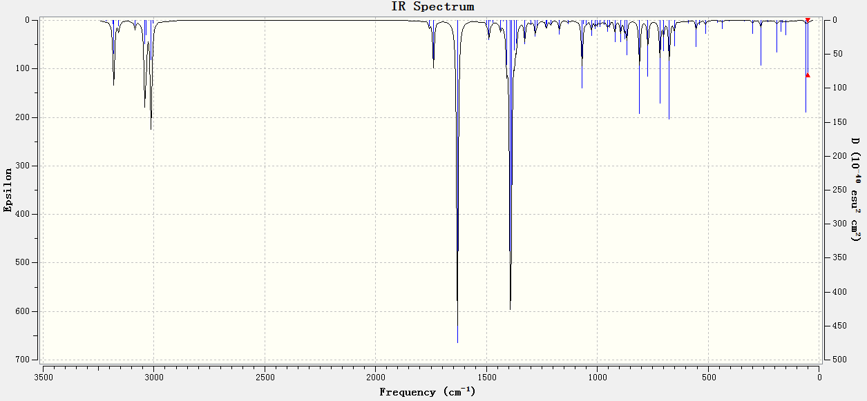
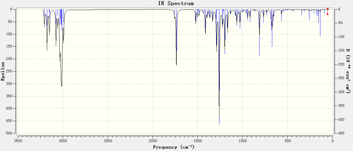
| Molecule; type of spectrum | 4a; 13C | 4a; 1H | 4b; 13C | 4b; 1H |
|---|---|---|---|---|
| Output spectrum |  |
 |
 |
 |
Conclusion
It has been shown that use of spectroscopic methods in identifying the difference between two isomers is indeed effective. Through energy minimisations and the examination of associated molecular orbitals, the reasoning behind the marked stability of 4a relative to 4b has also been explored in depth. Finally, the comparisons between calculated and literature spectral data yielded mixed results. Whilst the carbon spectrum was able to serve as a clear differentiator between the two compounds, the proton NMR, whilst primarily agreeing with previous values, was not as conclusive.
References
- ↑ N.L. Allinger, J. Am. Chem. Soc., 1977, 99, pp 8127-8134 DOI:10.1021/ja00467a001
- ↑ T.A. Halgren, J. Comput. Chem., 1996, 5-6, pp 490-519 DOI:<490::AID-JCC1>3.0.CO;2-P 10.1002/(SICI)1096-987X(199604)17:5/6<490::AID-JCC1>3.0.CO;2-P
- ↑ W. Herndon, C. Grayson, J. Manion. J. Org. Chem., 1967, 32(3), pp 526–529 DOI:10.1021/jo01278a003
- ↑ P. Caramella et. al, J. Am. Chem. Soc., 2002, 124(7), pp 1130 1131 DOI:10.1021/ja016622h
- ↑ J. Garcia et. al, Acc. Chem. Res., 2000, 33(10), pp 658–664 DOI:ar0000152 10.1021/ ar0000152
- ↑ J.A. Berson, E.J. Walsh Jr.,J. Am. Chem. Soc., 1968, 90(17), pp 4729–4730 DOI:10.1021/ja01019a040
- ↑ A. Greenberg et al., J. Am. Chem. Soc., 1996, 118(36), pp 8658-8668 DOI:10.1021/ja960294h
- ↑ L. Paquette et al., J. Am. Chem. Soc., 1990, 112, 277-283. DOI:10.1021/ja00157a043
- ↑ S.P. McGlynn et al., J. Phys. Chem., 1962, 66(12), pp 2499–2505, DOI:10.1021/j100818a042
- ↑ U. Brinker et al., J. Org. Chem., 2012, 77, 3800-3807 DOI:10.1021/jo3001035
- ↑ R. Gleiter; R. Hoffmann, J. Am. Chem. Soc., 1968, 90, 5457 DOI:10.1021/ja01022a023
- ↑ J. Mieusset et al., J. Am. Chem. Soc., 2008, 130, 14634 DOI:10.1021/ja8042118
- ↑ J. Neff; J. Nordlander, J. Org. Chem., 1976, 41, 2590 DOI:10.1021/jo00877a017
- ↑ R. Yang; L. Dai, J. Org. Chem., 1993, 58(12), pp 3381–3383 DOI:10.1021/jo00064a027