Year 3 Computational Labs

Molecular Dynamics Simulations of Simple Liquids

Abstract

Fill

Introduction

Fill

Aims and Objectives

Fill

Methods

In order for the simulation to replicate a real system as accurately, a few criterion had been defined, namely the simulation model, initial test parameters, forcefield, final parameters and tools used.

Velocity-Verlet Algorithm and Timestep

Using approximations, we assumed that atoms will behave classically and therefore the velocity-Verlet algorithm was applied into the simulation, where we have defined the starting positions of the atoms, x_i(0) and their velocities at the same time, v_i(0). As an example, this algorithm was used in a simple harmonic oscillator: https://goo.gl/As44o7

A timestep of 0.1 was initially tested. Subsequently, the value of "ERROR" as function of time was investigated and was found that this relationship was given by:

y = 0.000422x + 0.000073

R-squared value = 0.999977

The function above remained constant although the value of timestep was varied. It was found that when timestep was increased, this will add more cycles to the "ENERGY" and "ERROR" graphs but period remained constant. Amplitude of "ERROR" graph will increase over time leading to bigger magnitude in error. However, the function of maxima in the "ERROR" graph was unchanged. The "ENERGY" graph will also have higher amplitude, hence bigger change in total energy. Timestep must therefore not exceed 0.1990665 for change in total energy to remain below 1%.

The prove of concept is shown here: https://goo.gl/zC9YU9

Moreover, the total energy of a physical system was measured and expected to remain constant, indicating that the system has completed equilibration and energy has been completely redistributed among the particles in a given system (through collisions) upon the start of the simulation.

Model

A simple particle in a box model was used for all of the simulations. Using LAMMPS, a cubic box of a given length containing a given amount of atoms of mass 1.0 was created. This will form the boundary for the simulations carried out.

For atoms that move beyond this boundary, the periodic boundary conditions was able to correct the atoms' coordinates by allowing its replica to enter from the opposite face.

For instance, an atom at position (0.5, 0.5, 0.5) in a cubic simulation box which runs from (0, 0, 0) to (1.0, 1.0, 1.0), moving along a vector (0.7, 0.6, 0.2) in a single timestep, its final position is at (1.2, 1.1, 0.7). But after applying periodic boundary conditions, the atom position was corrected to (0.2, 0.1, 0.7).

To give an idea of the number of molecules simulated, the number of moles of 1 ml of water under standard conditions were estimated:

m of 1 ml water = ρV = 1 g

n of 1ml water = m/M_r = 0.05550843506 mol

Number of water molecules = nN_A = 3.342796 x 10²²

This is a large and unsuitable number to simulate. A value of 10000 would be more reasonable, thus the volume of 10000 water molecules was calculated to give a better perspective:

For 10000 water molecules, n of water = n.o.m./N_A = 1.660539 x 10^-20 mol

m of water = nM_r = 2.991507 x 10^-19 g

V of water = m/ρ = 2.991507 x 10^-19 ml

Forcefield

The Lennard-Jones potential, which fits well into the physic of the simulation, was utilised knowing that the force acting on the atoms depended on the potential they experienced. At longer distances however, this interaction will be so small that it can be negligible, so a cutoff point of 3.0σ was put in place.

Lennard-Jones Potential, U = 4ε [(σ/R)¹²-(σ/R)⁶]

To understand the relationship better, the separation r₀ at which the potential of zero was evaluated:

When U=0, (σ/R)¹²-(σ/R)⁶ = 0

Let (σ/R)⁶ = y, thus y²-y = 0, y(y-1) = 0

Therefore, y=0, (σ/R)⁶ = 0, undefined; (y-1)=0, (σ/R)⁶= 1, hence R=r₀=σ (F = repulsive force)

Along with the separation at equilibrium and hence the well depth ϕ(r_eq),

At equilibrium, F=0 (minimum), dU/dR = -48εσ¹²(1/R¹³) + 24εσ⁶(1/R⁷)

For turning point, dU/dR = 0

Thus, 24εσ⁶(1/R⁷) = 48εσ¹²(1/R¹³), (1/R⁷) = 2σ⁶(1/R¹³)

(1/R⁷)/(1/R¹³) = 2σ⁶, R⁶=2σ⁶, hence R=(₆√2)σ, R=r_eq=1.12246σ

Therefore well depth, ϕ(r_eq) = 4ε [(σ¹²/(₆√2)¹²σ¹²) - (σ⁶/(₆√2)⁶σ⁶)]

ϕ(r_eq) = 4ε [(1/4)-(1/2)], ϕ(r_eq) = -ε (minimum)

Moreover, the values of integrals of 2 σ, 2.5 σ and 3 σ to infinity were calculated respectively:

∫ϕ(r)dr = -1/3εσ¹²(1/R¹¹) + 2/3εσ⁶(1/R⁵), and when σ=ε=1,

For 2 σ, ∫ϕ(r)dr = -1/3(1)(1)¹²(1/2¹¹) + 2/3(1)(1)⁶(1/2⁵) = 0.020671

For 2.5 σ, ∫ϕ(r)dr = -1/3(1)(1)¹²(1/2.5¹¹) + 2/3(1)(1)⁶(1/2.5⁵) = 0.0068127

For 3 σ, ∫ϕ(r)dr = -1/3(1)(1)¹²(1/3¹¹) + 2/3(1)(1)⁶(1/3⁵) = 0.0027416

Reduced Units

The quantities used in the simulation were treated and divided with a scaling factor, such as σ or ε, to ensure that our results were more manageable. For example, for argon with Lennard-Jones (LJ) parameters σ = 0.34nm and ε/k_B = 120K, its LJ cutoff r* = 3.2 in real units was:

r=r*σ

r = 3.2(0.34 x 10^-9) = 1.088 x 10^-9 m

Thus, its well depth in real units was:

ϕ(r_eq) = ε = k_BT x N_A

ε = (1.38065 x 10^-23 JK^-1)(120 K)(6.02214 x 10²³mol^-1) = 997.73546 J mol^-1 = 0.997735 kJ mol^-1

Also, the reduced temperature T* = 1.5 can be calculated in real units:

T = T*ε/k_BN_A

T = 1.5(997.73546 J mol^-1)/(1.38065 x 10^-23 JK^-1)(6.02214 x 10²³ mol^-1) = 180 K

Lattice Structure

Giving atoms random starting coordinates can be problematic as this may generate two atoms close to each other in our simulation, where if the separation between them was below σ, this can cause a strong (or even infinite) repulsion pushing the atoms apart. Therefore, the atoms were initially created in a 3D simple cubic (sc) lattice.

Given that the number density (N/V) of lattice points was 0.8, the lattice spacing was found to be:

Number density, ρ=N/V, V=N/ρ

V = 1/0.8 = 1.25

Lattice spacing, l = ₃√1.25 = 1.07722

Also for a face-centred cubic (fcc) lattice with number density 1.2, its lattice spacing was calculated:

V=N/ρ = 4/1.2 = 3.33333

Lattice spacing, l = ₃√3.33333 = 1.49380

Furthermore, a simulation sc box of width 10 was created as a control. Within this region, there were 4000 atoms present (4 atoms in each unit cell where there are 10x10x10 = 1000 unit cells). Following this, the mass and pair coefficient of the each type of atom were assigned as below:

mass 1 1.0

pair_style lj/cut 3.0

pair_coeff * * 1.0 1.0

Definitions for each line in the command code are provided as such:

mass 1 1.0

Description: Assigning mass of value 1.0 to all type 1 atoms

pair_style lj/cut 3.0

Description: Specifying a standard 12/6 Lennard-Jones potential with no Coulomb between atom pairs with global LJ cutoff set to distance r*=3.0

pair_coeff * * 1.0 1.0

Description: Setting the pairwise forcefield coefficients for the symmetric I,J interaction to the same value of 1.0 for all (given by asterisk) type 1 with type 1 atom pairs

Timestep Optimisation

The code below was written in the input script with the timestep taking a value of 0.001:

### SPECIFY TIMESTEP ###

variable timestep equal 0.001

variable n_steps equal floor(100/${timestep})

timestep ${timestep}

### RUN SIMULATION ###

run ${n_steps}

run 100000

Note: The variable command is a loop which was assigned a value that is later evaluated in the input script, where in this case timestep was equal to 0.001. This is useful because the defined value can be referenced in subsequent variables, therefore making it reusable and eliminating the need to repeatedly input the value 0.001. For instance, the defined timestep was used in the math function "floor" assigned to variable n_step and subsequently the value n_step is used in the "run" command. Hence, this coding method will be more pragmatic than just writing the script simply as:

timestep 0.001

run 100000

Choosing the correct timestep was crucial for the subsequent simulations which were undertaken. To determine the optimum timestep, simulations using different timesteps (0.001, 0.0025, 0.0075, 0.01 and 0.015) were tested. To illustrate that the simulation had equilibrated, the graphs of total energy, temperature and pressure against time were plotted for the 0.001 timestep experiment:

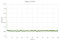Figure 1: Total energy against time plot for timestep 0.001

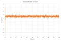Figure 2: Temperature against time plot for timestep 0.001

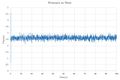Figure 3: Pressure against time plot for timestep 0.001

From the plots above, the simulation did achieve equilibrium and the values of total energy, temperature and pressure had converged to a constant average (within a certain degree of error) at approximately 0.5 s into the simulation.

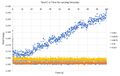Figure 4: Single plot of total energy against time for all five timesteps.

Among the five timesteps, 0.001 was most likely to give acceptable results. The data obtained was of high resolution, with the smallest interval between data points. The simulation was said to give the best representation of a physical reality being investigated. On the other hand, a timestep of 0.015 was the least suitable choice because the total energy does not converge. The energy initially stabilised but subsequently diverged (increased) after 20 s and thus system has not fully equilibrated. To give the best balance between resolution and speed (time taken to complete a simulation), timestep within the acceptable range of 0.001 to 0.003 were used. Any timestep above 0.003 would not properly allow for total energy to converge and gives a large gap between data points.

LAMMPS Toolkit

The LAMMPS Molecular Dynamics Simulator is an extremely useful simulation software containing a vast array of tools that was further utilised throughout this experiment. Among them were the "variable" and "thermo_style" commands used in changing ensembles and measuring thermodynamics properties respectively, which were crucial in obtaining key data. Towards the end of the investigation, the usage of the radial distribution function (RDF), mean squared displacement (MSD) and velocity autocorrelation function (VACF) were also explored and applied into many of the simulations conducted.

Visual Molecular Dynamics (VMD)

To help visualise some of the simulations, LAMMPS was also supported by the VMD 3D graphics programme that was able to read trajectory (.trj) files in order to display our simulation through multiple modes and perspectives. This software was also used to conduct further calculations such as evaluating running integrals for the RDF.

Results and Discussion

NpT Ensemble

For this section of the investigation, the simulation has been modified so that it can run under NpT conditions (called the isobaric-isothermal ensemble in statistical mechanics) to understand what changes to thermodynamic properties occur at this particular experimental condition. The data collected was used to plot an equation of state at atmospheric pressure for the case of our model fluid.

Five values of temperature (2.0, 2.5, 3.0, 3.5, 4.0) and two values of pressure (3.0, 4.0) given in Lennard-Jones units were chosen based on the results of the optimisation test ran earlier. The timestep was set to 0.0025 and the input script modified accordingly for all ten (p,T) phase points before being submitted to LAMMPS.

1. Controlling Temperature

In general, temperature, T at a given time during the course of the simulation will be prone to fluctuations and will differ slightly from the intended temperature of the system, 𝛕 (value specified in the input script). However, T can be easily controlled by multiplying each velocity term of each atom by a constant factor, γ whereby:

The kinetic energy of the system can be written as:

1/2m₁v₁² + 1/2m₂v₂²+ 1/2m₃v₃² = 3/2Nk_BT (Eq. 1)

1/2m₁(γv₁)² + 1/2m₂(γv₂)²+ 1/2m₃(γv₃)² = 3/2Nk_B𝛕 (Eq. 2)

Dividing (Eq. 2) by (Eq. 1):

(γ²v₁² + γ²v₂²+ γ²v₃²)/( v₁² + v₂²+ v₃²) = 𝛕/T

γ² = 𝛕/T, thus γ = √(𝛕/T)

Thus, the value of γ can be determined and used to correct any deviations in T.

2. Sampling and Averaging

In the input script, there were lines entered as:

fix aves all ave/time 100 1000 100000 v_dens v_temp v_press v_dens2 v_temp2 v_press2
run 100000

These lines were needed to measure key thermodynamics properties such as density, temperature and pressure respectively. Most importantly, the values 100, 1000 and 100000 play a vital role in directing how often these properties are averaged and how many measurements contribute to the final average. Each number is represented as follows:

100 = Nevery

1000 = Nrepeat

100000 = Nfreq

The three arguments above specify the timesteps the input values will be used in order to contribute to the average. The final averaged quantities are generated on timesteps that are a multiple of 100000. The average was over 1000 quantities, computed in the preceding portion of the simulation every 100 timesteps. Nfreq must be a multiple of Nevery and Nevery must be non-zero even if Nrepeat was 1. Also, the timesteps contributing to the average value cannot overlap, i.e. Nrepeat*Nevery cannot exceed Nfreq.

Hence, by referring to the log (.log) output file, the amount of time that has been simulated for this investigation was 50 s.

3. Equation of State

The density of the system obtained from the log files were plotted against temperature for both of pressures that were simulated, including error bars. Also included in the graphs was a curve for the expected densities as predicted by the ideal gas law, pV =NkT.

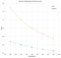Figure 5: Density as a function of temperature at pressure, p = 3.0

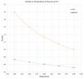Figure 6: Density as a function of temperature at pressure, p = 4.0

It was found that the simulated density was always lower than the values predicted by the ideal gas law for a given pressure. This was because for an ideal gas, there was no interactions between the atoms whereas the atoms in our simulation had been modeled using a forcefield of the Lennard-Jones potential. Moreover, the discrepancy between the observed and predicted values of density increased with pressure, especially at the lower temperatures where the deviation was larger.

NVT Ensemble

1. Heat Capacity

In a particular system where temperature was fixed, thermodynamic properties such as total energy were likely to fluctuate from its constant average and these fluctuations gives rise to the heat capacity, Cv where its value can be calculated using:

Cv = δE/δT = N².Var(E)/k_BT²

However, it was important to note that the simulation carried out here was altered to NVT conditions (canonical ensemble). As with the previous simulation, ten phase points were required, but this time using five values of temperature (2.0, 2.2, 2.4, 2.6, 2.8) and two values of density (0.2, 0.8). A copy of the modified input script for NVT is attached below to highlight the changes made:

https://goo.gl/5GnrfV

2. Results

Once data was collected from the log files (but without standard errors), the graph of Cv/V against average temperature was plotted on the same axes, where V was the volume of the simulation cell.

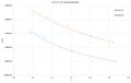Figure 7: A plot of heat capacity over volume as a function of average temperature

From the results obtained, this was not the trend that was expected. The data supposed to show a constant heat capacity for both densities, but instead heat capacity decreases when temperature was increased. Comparing both sets of data, for a system having a higher density, its heat capacity will in turn be raised.

Radial Distribution Function (RDF)

The radial pair distribution function or g(r) is defined as the probability of locating the nearest neighbouring atom at a distance r from a reference atom. The visualising software VMD was used to calculate the RDF of three simulations under different states, that were the solid, liquid and vapour phases.

1. Phase Transitions

In order to set up the various states, the values of density and temperature of the simulation were modified appropriately based on the phase transitions of the Lennard-Jones system. The following were the set of parameters determined for each state:

Solid: Lattice fcc, density = 1.4, T = 1.5

Liquid: Lattice sc, density = 0.8, T =1.5

Vapour: Lattice sc, density = 0.01, T = 1.0

A timestep of 0.002 was used to run all simulations in LAMMPS.

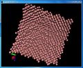Figure 8(a): View of solid phase simulation in VMD

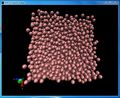Figure 8(b): View of liquid phase simulation in VMD

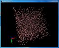Figure 8(c): View of gas phase simulation in VMD

2. Qualitative Analysis of RDF

When each simulation was completed, its .trj file was inputted into VMD where the value of g(r) and ∫ g(r) dr (or running integral) were evaluated. The graph of RDF against reduced distance were plotted on the same axes for all three states.

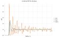Figure 9: Combined g(r) against reduced distance plot for the solid, liquid and vapour systems

In the s

olid RDF, the function showed a regular pattern of peaks with almost the similar intervals over a long range of distance. The peaks were discrete at approximately σ, √2 σ, √3 σ, and so on. There was a very high chance of finding an atom at the position of these peaks whilst the probability of locating an atom between the peaks was very low. This illustrated that solids had a uniform packing structure and had very little defect within the lattice. Moreover, the first three peaks corresponded to the first, second and third coordination shells.

Thus the lattice spacing can be determined:

V=N/ρ = 4/1.4 = 2.85714

Lattice spacing, l = ₃√2.85714 = 1.41898

To calculate the coordination number, g(r) was integrated in spherical coordinates to the first minimum of the RDF. Hence, the coordination numbers for the solid were: first peak (12), second peak (4), and third peak (8).

For the liquid RDF, the first and sharpest peak occured close to σ and the subsequent peaks appeared at about intervals of σ, but smaller than the first peak. At longer distances of r, the value of g(r) remained unchanged at 1, showing that liquid particles were independent of one another. Thus, liquids were less closely packed compared to solids and had the ability to move dynamically, hence they do not possess a fixed structure. They were able to form multiple coordination spheres, but in most cases, there was only one coordination sphere present at a given time.

In the vapour RDF, the function only showed one obvious peak at about σ which then plateaued off at a value of g(r) = 1, the normal bulk density of the system. The regions that experienced the greatest intermolecular forces when g(r) > 1 were for 1 < σ < 2.5. From this result, it was concluded that gases tend to move around randomly in a sporadic motion (Brownian motion) and at most, they only have a single short-lived coordination sphere.

Diffusion Coefficient

In this experiment, the way in which atoms move around in the system (through translational motion) was of particular interest. This form of motion was governed by the diffusion coefficient, D or mass diffusivity, which can be measured using two main methods detailed below:

1. Mean Squared Displacement (MSD)

Since D was closely related to MSD, a simulation was ran (at specific density and temperature) for all three phases with an additional input command to calculate MSD and VACF (mentioned in next section). The set of parameters used to obtain each physical phase were identical those implemented during the RDF investigation:

Timestep = 0.002

Solid: Lattice fcc, density = 1.4, T = 1.5

Liquid: Lattice sc, density = 0.8, T =1.5

Vapour: Lattice sc, density = 0.01, T = 1.0

Once data was obtained from the "optional output-2" files, the total MSD (resultant MSD from individual Cartesian directions (x,y,z)) was plotted against timestep:

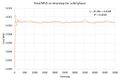Figure 10(a): Total MSD as a function of timestep for the solid phase

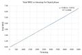Figure 10(b): Total MSD as a function of timestep for the liquid phase

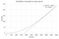Figure 10(c): Total MSD as a function of timestep for the gas phase

The relationship between total MSD and timestep obtained for the three phases were as expected. Total MSD for solids initially fluctuated before becoming constant whereas for the liquid phase, its values increased linearly but gradually, and as for the vapour phase, total MSD increased linearly and rapidly.

Since D = 1/6 δ<r²(t)> / δt, then D = 1/6 (gradient of graph of MSD vs timestep).

Thus using the gradient of the best-fit line, for:

Solid: D = 1/6 (2.3514 x 10^-8) = 3.919 x 10^-9 s^-1

Liquid: D = 1/6 (1.3140 x 10^-3) = 2.190 x 10^-4 s^-1

Vapour: D = 1/6 (7.2313 x 10^-2) = 1.205 x 10^-2 s^-1

With this, the diffusion coefficient was shown to have increased going from solids to gases. Moreover, it was noted that the diffusion coefficient for the solid phase was so small, it was negligible (zero).

2. MSD: One Million Atoms

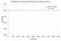Figure 11(a): Total MSD plotted against timestep for the solid phase for simulation containing one million atoms

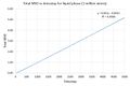Figure 11(b): Total MSD plotted against timestep for the liquid phase for simulation containing one million atoms

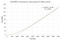Figure 11(c): Total MSD plotted against timestep for the solid phase for simulation containing one million atoms

For the same simulation repeated using one million atoms, values of total MSD obtained were higher compared to that with fewer atoms (except for the solid phase where the total MSD was lowered). Moreover, total MSD for the liquid and vapour phases increased more linearly when using more atoms (and this was most evident for the vapour phase). Hence, the gradient of the best-fit line was used to evaluate the values of D as shown below:

Solid: D = 1/6 (5.26956 x 10^-8) = 8.783 x 10^-9 s^-1

Liquid: D = 1/6 (1.04717 x 10^-3) = 1.745 x 10^-4 s^-1

Vapour: D = 1/6 (3.57206 x 10^-2) = 5.953 x 10^-3 s^-1

Overall, the same trend was observed, with the addition that the diffusion coefficients for the liquid and gas systems were slightly lower than before.

3. Extension: Velocity Autocorrelation Function (VACF)

The other alternative way of calculating D was by using the velocity autocorrelation function. The same input script was used here (as in the previous MSD section) and the simulation was ran for the solid, liquid and vapour phases. All data was obtained from the "optional output-3" files.

In relation to the theoretical concepts covered in the 1D harmonic oscillator, the normalised velocity autocorrelation function, C(τ) was evaluated for this 1D harmonic system:

Given that C(τ) = < v(t).v(t+τ) > and x(t) = cos(ωt+ϕ),

VACF of a 1D harmonic oscillator, C(τ) = ∫ v(t).v(t+τ) dt

Thus, the normalised VACF, C(τ) = ∫ v(t).v(t+τ) dt / ∫ v(t)² dt

Hence to compare between the different oscillating systems, the graph of C(τ) with ω=1/(2п) along with the VACFs from the solid and liquid simulations was plotted along the same axes, from x = 0 to 500.

Figure 12: C(τ) with ω=1/(2п) and the VACFs of the solid and liquid phases as a function of timestep (x = 0 to 500)

In the solid and liquid phases, where atoms are close to each other and of high density, strong interatomic forces were most evident. Atoms in these systems tend to adopt a position where there was a balance between the attractive and repulsive forces, thus they will not be easily displaced. As a result, these atoms will oscillate as part of their motion, vibrating between points of maxima and minima. Hence, this gave rise to a VACF function which showed a periodic oscillation from positive to negative values.

For the case of solids, the magnitude of oscillation decayed over time due to forces acting to oppose these motion, thus the function closely resembled a damped oscillation that decreased exponentially. Whilst for liquids, the atoms behaved similarly but they were able to glide among themselves. The process of diffusion also drastically weakened any oscillatory motion the system possessed and the VACF function showed a very damp oscillation, with only a single minima point.

Note: The minima in the VACFs in the solid and liquid system relates to the maximum change in the magnitude or direction (of the atoms in the system), thus altering their velocities, giving rise to a minimum value for the product of v(t=0) and v(t=τ).

On the other hand, the 1D harmonic oscillator model has a VACF function of constant amplitude (A=1) and period (T=40 s). Its magnitude of oscillation was greater than that of the solid and liquid systems, implying that no damping or perturbative forces had acted upon the system throughout its motion (and based on Newton’s Law of Motion the oscillation its motion will not change and continue to remain this way). Whereas, unlike the Lennard-Jones model describe earlier, atoms in the 1D harmonic oscillator do not interact with each other by attraction or repulsion and thus no energy was dissipated.

4. The Trapezium Rule

Utilising the trapezium rule (TR) to approximately calculate the integral or area under the VACF graph, the values of D were estimated for each of the three physical phases.

Given D = 1/3 ∫ <v(0).v(τ)> dτ, then D = 1/3 (area under the graph of C(τ) vs timestep).

Thus using the area under the graph obtained by the TR, for:

Solid: D = 1/3 (216.9089038) = 72.303 s^-1

Liquid: D = 1/3 (277.865793) = 92.622 s^-1

Vapour: D = 1/3 (10675.4021) = 3358.467 s^-1

The values of D above were as expected, with it increasing in magnitude from the solid to vapour phase. Going a step further, the running integrals for each case were also evaluated (once again using the TR) and plotted as a function of timestep as follows:

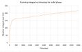Figure 13(a): Graph of number integral of C(τ) against timestep for the solid phase

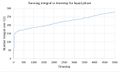Figure 13(b): Graph of number integral of C(τ) against timestep for the liquid phase

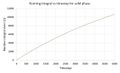Figure 13(c): Graph of number integral of C(τ) against timestep for the gas phase

The running integral for the solid and liquid phases were almost identical, having a rapid increase at the start and leveling off towards the end (due to atomic oscillations and small fluctuations in velocity). For gases on the other hand, its running integral increases gradually as a result of the exponential decay trend seen in its C(τ) against timestep plot. Thus, in statistical mechanics term, it can be concluded that the velocity has decorrelated with time showing the presence of weak forces becoming prominent in the vapour system.

5. VACF: One Million Atoms

The same procedures described above were applied for the simulation containing one million atoms, and thus for:

Solid: D = 1/3 (176.9191107) = 58.973 s^-1

Liquid: D = 1/3 (151.586442) = 50.529 s^-1

Vapour: D = 1/3 (4902.698696) = 1634.233 s^-1

As such, the values of diffusion coefficient increased from the solid to vapour phase as predicted, but was anomalous for the liquid phase (a decrease from the trend).

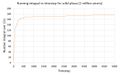Figure 14(a): Graph of number integral of C(τ) against timestep for solids for 1 million atoms

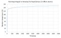Figure 14(b): Graph of number integral of C(τ) against timestep for liquids for 1 million atoms

Figure 14(c): Graph of number integral of C(τ) against timestep for gases for 1 million atoms

As with the simulation using fewer atoms, the running integral plots for one million atoms were consistent in its trend. One difference was that the final integral (or maximum height) for the solid and liquid phases were lower than before, indicating that the magnitude of oscillation of atoms in the system had decreased and there were smaller fluctuations. For the vapour phase, there was a more evident exponential trend, which better correlates the simulation with the real system.

Conclusion

Fill

References

Fill