Rep:Mod:dt2315MC2DIM

Introduction to the Ising Model

The Model

• The lowest energy configuration

This is achieved in a parallel alignment of the magnetic spins. If $s_i=+1$ is spin up and $s_i=-1$ is spin down, the energy can be calculated as:

$$\begin{gathered} E=-\frac{1}{2}J\sum _i^N\sum _{j \\ \in \\ \mathrm{n}\mathrm{e}\mathrm{i}\mathrm{g}\mathrm{h}\mathrm{b}\mathrm{o}\mathrm{u}\mathrm{r}\mathrm{s}\left(i\right)}{s}_i{s}_j \end{gathered}$$

The energy is minimum when the sum is maximised. This happens when the $s_i{s}_j=+1$ so the all the spins must be the same–either all spin up or down. It is should be noted that the number of spin interactions is 2 x the number of dimensions (i.e. each spin interacts with 2 in 1D, with 4 spins in 2D and 6 spins in 3D).

In that case, the formula can be simplified as follows, where $D$ is the number of dimensions and $N$ is the total number of spins:

$$\begin{gathered} E=-\frac{1}{2}J\sum _i^N\sum _{j \\ \in \\ \mathrm{n}\mathrm{e}\mathrm{i}\mathrm{g}\mathrm{h}\mathrm{b}\mathrm{o}\mathrm{u}\mathrm{r}\mathrm{s}\left(i\right)}{s}_i{s}_j=-\frac{1}{2}J\sum _i^N \\ 1*2D=-DNJ \end{gathered}$$

Example: In 1D and N = 5, if all the spins are spin up, each interaction $s_i{s}_j=+1$ so $E=-J(1+2/2+2/2+2/2+1)=-5J$. Note: if first and last spin are considered to only interact once so there is no need to half the interactions. The same result would be obtained using: $$\begin{gathered} E \\ = \\ -DNJ=-1*5*J=-5J \end{gathered}$$

• Multiplicity of the lowest energy state

The multiplicity is given by combinations of the N spins available. The spins can either be all up or all down in this configuration and spins are indistinguishable from each other, so the multiplicity is:

$M=2$

• Entropy of the lowest energy state

$S=k_{b}lnM=k_{b}ln2=9.57*10^{-24}J{K}^{-1}$

Phase Transitions

Change in spin

If the system is in the lowest energy configuration (i.e. all spins up or all down), in order to move to a different state, one of the spins must spontaneously change direction. The change in energy and the change in entropy are calculated for a lattice with $$\begin{gathered} D=3, \\ N=1000 \end{gathered}$$.

• Change in energy

The spin that is flipped leads to 6 spin interactions that increase the energy (in 3D).

$E_0=-DNJ=-3*1000*J=-3000J$

$E_1=-D(N-1)J+1*6*J=-3*999*J+6J=-2991J$

$\mathrm{\Delta }E=E_1-E_0=-2991J+3000J=9J$

• Change in entropy

The entropy gained by the system is given by:

$S_0=k_{b}lnM=k_{b}ln2=0.095*10^{-22}J{K}^{-1}$ - 2 state possible with all spins up/down

$S_1=k_{b}lnM=k_{b}ln(2*N)=k_{b}ln2000=1.049*10^{-22}J{K}^{-1}$ - if one spin is up it can take any of the 1000 positions; same for on spin down

$\mathrm{\Delta }S=S_1-S_0=(1.049-0.095)*10^{-22}=0.954*10^{-22}J{K}^{-1}$

The entropy increased 10 times by only flipping one spin.

Magnetisation

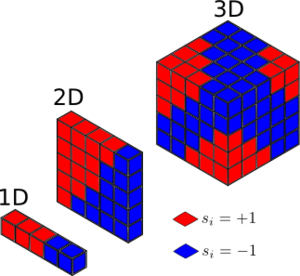
The magnetisation is calculated for the 1D and 2D lattices shown below.

• 1D

$M=\sum _i{s}_i=3*(+1)+2*(-1)=+1$

• 2D

$M=\sum _i{s}_i=13*(+1)+12*(-1)=+1$

• Ising lattice with $$\begin{gathered} D=3, \\ N=1000 \end{gathered}$$ at absolute 0 K

At absolute 0 the lattice is in the region below the critical temperature and shows ferromagnetic behaviour. As a result, the magnetisation would be expected to maximum (absolute value).

If all spins are up:

$M=\sum _i{s}_i=(+1)*1000=+1000$

If all spins are down:

$M=\sum _i{s}_i=(-1)*1000=-1000$

Calculating the energy and magnetisation

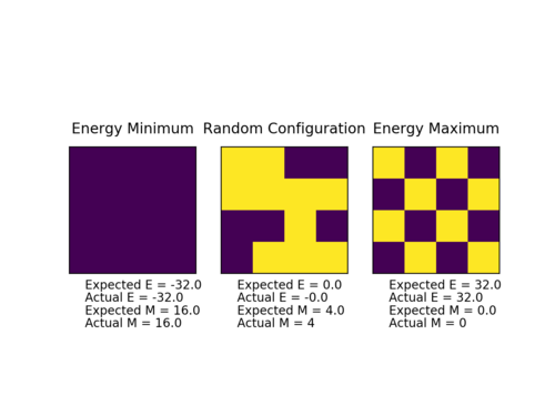
The energy was calculated in $J=k_B$ units and the results of the ILcheck.py script are shown below.

Introduction to the Monte Carlo simulation

• 100 spins system

For a system with 100 spins, such as a 10x10 2D lattice for which it is generously assumed that $1\times 10^9$ configurations can be analysed per second, the time to evaluate a single value of the magnetisation at one particular temperature can be estimated:

Number of possible configurations: $2^{100}$

Estimated time: $10^{30}/10^9=10^{21}$ seconds or more than $10^{13}years$

A quicker way is obviously needed and Importance sampling is used by neglecting the states which are very unlikely to occur (i.e. vanishingly small Boltzmann factor). A montecarlocycle(T) function is presented below. The function returns the energy (in units of $k_B$) and the magnetisation of the lattice at the end of the cycle.

def montecarlostep(self, T):
        #the function performs a single Monte Carlo step
        E_0 = self.energy()
        #two random coordinates are selected to choose a spin
        random_i = np.random.choice(range(0, self.n_rows))
        random_j = np.random.choice(range(0, self.n_cols))
        #one random number in the range[0,1) is generated
        random_number = np.random.random()
        self.lattice[random_i, random_j] = -(self.lattice[random_i, random_j])
        E_1 = self.energy()
        d_E = E_1 - E_0
        if d_E <= 0:
            pass
            #configuration with spin flipped accepted
        else: 
            if random_number <= np.exp((-d_E)/T):
                pass
                #configuration with spin flipped accepted
            else:
                self.lattice[random_i, random_j] = -(self.lattice[random_i, random_j])  
                #configuration with spin flipped rejected and spin is flipped back
        self.n_cycles += 1
        if self.n_cycles > self.N:
        #the values are changed only after the number of cycles that are chosen to be ignored for each lattice
            self.E += self.energy()
            self.E2 += self.energy()**2
            self.M += self.magnetisation()
            self.M2 += self.magnetisation()**2
        else:
            pass
        energy = self.energy()
        magnetisation = self.magnetisation()
        #the function returns the energy and magnetisation of the current lattice (not the total ones)
        return energy, magnetisation

def statistics(self):
        #the function calculates the values for the averages of E, E*E (E2), M, M*M (M2), and returns them
        return self.E/(self.n_cycles - self.N), self.E2/(self.n_cycles - self.N), self.M/(self.n_cycles - self.N), 
        self.M2/(self.n_cycles - self.N), self.n_cycles

• Reaching an equilibrium state at $T<T_C$

Below the Curie Temperature, equilibrium can be reached in two ways: all the spins have the same orientation OR the spins cancel out overall and there are magnetic regions (Weiss domains) within which the magnetisation is in a uniform direction. In both situations, the magnetisation is expected to be 0. However, if there is enough thermal energy, some spins could randomly flip, but shortly re-equilibrate and the average $⟨M⟩\ne 0$ is expected to be 0.

The two equilibrium situation are shown below with the output from the statistics() function. It should be noted that the average magnetisation is not 0 as the configurations at the beginning of the simulations are taken into account.

Averaged quantities for equilibration with spins in the same orientation:

E =  -1.68658447266

E*E =  3.02299118042

M =  -0.816345214844

M*M =  0.730360031128

Averaged quantities for equilibration with 3 magnetic regions:

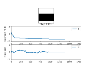
E =  -1.31509433962

E*E =  1.79771029874

M =  0.0245479559748

M*M =  0.00829218258648

Accelerating the code

The results of the ILtimetrial.py are given below for 10 repeats in each case

• 2000 Monte Carlo steps before optimisation

$7.58\pm 0.15$ seconds

• 2000 Monte Carlo steps after optimisation

$0.42\pm 0.01$ seconds

The duration of the simulation has become 18 times shorter by removing the double for loop and the functions used are provided below.

magnetisation = np.sum(self.lattice)

S += np.sum(np.multiply(self.lattice, np.roll(self.lattice, 1, axis = 1))) #rolls the last column in front of the lattice 

S += np.sum(np.multiply(self.lattice, np.roll(self.lattice, 1, axis = 0))) #rolls the last row at the top of the lattice 

energy = - self.J * S

Note: no 1/2 factor is needed as the spin interactions are only counted once.

The effect of temperature

• Equilibrium data

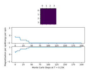
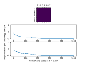
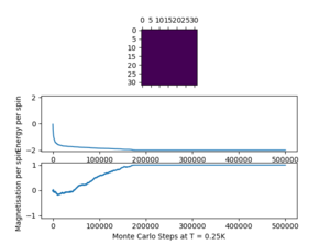
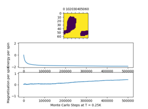
The script ILfinalframe.py was run at T = 0.25 K, and the plots are presented below. A low temperature below the critical temperature was chosen as the system takes longer to equilibrate at low temperatures, with less thermal energy. For each lattice size, a number of N cycles was ignored in the calculation of averages. It can be seen how the first steps which do not reflect the equilibrium situation can strongly affect the average values. Consequently, the statistics() and montecarlostep() functions were modified.

Lattice size	Cycles ignored	Running time	# repeats
2 x 2	20	500	5
4 x 4	100	5000	5
8 x 8	500	10,000	5
16 x 16	10,000	200,000	5
32 x 32	200,000	500,000	5
64 x 64	500,000	1,000,000	3

2x2	4x4	8x8

16x16	32x32	64x64

• Energy and Magnetisation for an $8\times 8$ lattice

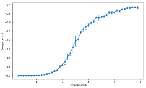
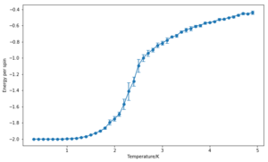
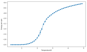
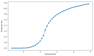
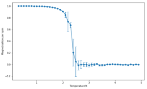
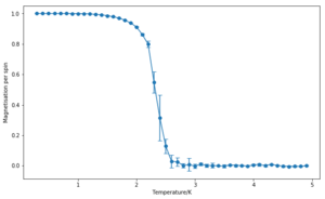
For this size, 500 cycles were ignored and the error bars shown in the graphs below give the standard deviation calculated for 5 repeats. The temperature range tested was 0.3 to 5.0, with a spacing of 0.1. It is expected that the error bars for energy are smaller than the ones for magnetisation since the system strives to achieve the minimum energy configuration, while the process of spin flipping is more random and different configurations with the same energy can be achieved.

The effect of system size

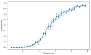
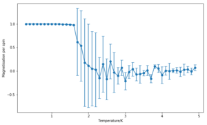
The calculation of energy and magnetisation was repeated for a range of lattice sizes and the corresponding number of cycles were removed. As expected, the error bars decrease with size. However, even for large systems like 32x32 or 64x64, the error bars are still large in the vicinity of the Curie Temperature. These correspond to the long range fluctuations caused by the random configurations that the system adopts after this point–the system goes from a ferromagnetic one to a paramagnetic one. While the bigger the lattice, the better the results are expected to be, the 32x32 lattice looks like it could provide a reasonable approximation, especially with an increased number of repeats.

2x2	4x4	8x8

16x16	32x32	64x64

Note: the simulation were run 5 times for all of the lattices apart from for the 64x64 which was only run 3 times.

Determining the heat capacity

Derivation

Definition of heat capacity:

$C=\frac{\partial ⟨E⟩}{\partial T}$

Definition of average energy and squared energy:

${⟨E⟩}_T=\frac{1}{Z}\sum _{\alpha }E\left(\alpha \right)\exp \{-\frac{E\left(\alpha \right)}{k_{B}T}\}$

${⟨E^2⟩}_T=\frac{1}{Z}\sum _{\alpha }{E}^2\left(\alpha \right)\exp \{-\frac{E\left(\alpha \right)}{k_{B}T}\}$

Definition of partition function:

$Z=\sum _{\alpha }E\left(\alpha \right)\exp \{-\frac{E\left(\alpha \right)}{k_{B}T}\}$

${⟨E⟩}_T>$ can be differentiated using the product rule as follows $(a*b{)}^{\prime }=a^{\prime }*b+a*b^{\prime }$ where $a=\frac{1}{Z}$ and $b=\sum _{\alpha }E\left(\alpha \right)\exp \{-\frac{E\left(\alpha \right)}{k_{B}T}\}$.

$\frac{\partial (1/Z)}{\partial T}=\frac{-1}{Z^2}\sum _{\alpha }\frac{E(\alpha )}{k_B{T}^2}\exp \{-\frac{E\left(\alpha \right)}{k_{B}T}\}$

$\frac{\partial \sum _{\alpha }E\left(\alpha \right)\exp \{-\frac{E\left(\alpha \right)}{k_{B}T}\}}{\partial T}=\sum _{\alpha }\frac{E^2\left(\alpha \right)}{k_B{T}^2}\exp \{-\frac{E\left(\alpha \right)}{k_{B}T}\}$

Using the results above:

$a^{\prime }*b=\frac{-1}{Z^2}\sum _{\alpha }\frac{E(\alpha )}{k_B{T}^2}\exp \{-\frac{E\left(\alpha \right)}{k_{B}T}\}*\sum _{\alpha }E\left(\alpha \right)\exp \{-\frac{E\left(\alpha \right)}{k_{B}T}\}=-\frac{1}{k_B{T}^2}{{⟨E⟩}_T}^2$

$a*b^{\prime }=\frac{1}{Z}*\sum _{\alpha }\frac{E^2\left(\alpha \right)}{k_B{T}^2}\exp \{-\frac{E\left(\alpha \right)}{k_{B}T}\}=\frac{1}{k_B{T}^2}{⟨E^2⟩}_T$

Using the definition of variance:

$\mathrm{V}\mathrm{a}\mathrm{r}[E]={⟨E^2⟩}_T-{{⟨E⟩}_T}^2$

$C=\frac{\mathrm{V}\mathrm{a}\mathrm{r}[E]}{k_B{T}^2}$

Comparison with C++ data

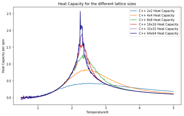
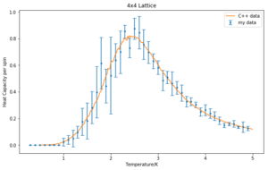
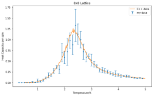
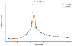
The average heat capacities from 5 runs and the corresponding error bars were plotted for each lattice in comparison with the given C++ data. They seem in relatively good agreement and the data should become more and more similar with an increased number of repeats. The heat capacity becomes strongly peaked close of the critical temperature and as the lattice size increases. Moreover, the Curie temperature changes with system size.

2x2	4x4	8x8

16x16	32x32	64x64

A plot of the heat capacities from the C++ data is shown to illustrate how heat capacity increases with size.

Locating the Curie Temperature

Polynomial fitting

The data for the 32x32 lattice was fitted as o polynomially. Different orders were tried and while the 15th order is one of the ones that works best, it is obviously still a poor fit.

Fitting in a particular temperature range

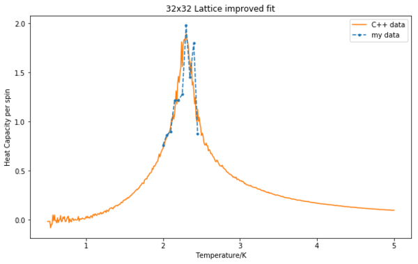
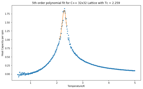
A much better fit was achieved by fitting the polynomial only to the peak of the heat capacity, on a temperature range between 2.1 K and 2.4 K. A comparison with the C++ data is shown and the values for the temperatures corresponding the the maximum heat capacity are given.

Finding the peak in C

• Estimate of $T_{C,\mathrm{\infty }}$

The temperature at which the maximum heat capacity occurs was plotted against 1/L for the C++ data for all the lattice sizes. As it can be seen, this temperature decreases with size and two fits are shown–one which using all the data and another one that only takes into considerations the 3 highest lattices. The estimate for $T_{C,\mathrm{\infty }}$ is given when 1/L goes to 0, so when the line crosses the y axis.

The value $T_{C,\mathrm{\infty }}=2.289K$ is slightly higher than the prediction of $2.269K$. However, $T_{C,\mathrm{\infty }}=2.271K$ significantly improves if only the larger sizes are used.

• Sources of error

The possible sources of error in calculating the Curie Temperature could be the fact that small size lattices are used. The results for my data are slightly higher and these should improve if more repeats are done, with longer running times and smaller temperature intervals in critical region.

This was tried with 4 additional runs for the 32x32 lattice on a temperature range between 2 and 2.4 with intervals of 0.05 K. It can be seen that this already provides a much better fit when compared to the C++ data.

Overall however, the results after 5 repeats show reasonable error bars and are quite similar to the C++ data.

References

1. H. A Kramers and G. H Wannier, "Statistics of the Two-dimensional Ferromagnet, Part I.", Physical Review, 60, 252, (1941).

2. A. E. Ferdinand and M. E. Fisher, "Bounded and Inhomogeneous Ising Models. I. Specific-Heat Anomaly of a Finite Lattice", Physical Review, 185, 832 (1969).

IsingLattice source code

import numpy as np

class IsingLattice:

    E = 0.0
    E2 = 0.0
    M = 0.0
    M2 = 0.0

    n_cycles = 1

    J = 1
    N = 200000
    #N = number of cycles ignored until energy and magnetisation become constant
    
    def __init__(self, n_rows, n_cols):
        self.n_rows = n_rows
        self.n_cols = n_cols
        self.lattice = np.random.choice([-1,1], size=(n_rows, n_cols))

    def energy(self):
        S = 0
        "Return the total energy of the current lattice configuration."
        "Code before optimization below"
        #N = self.n_rows
        #for i in range(self.n_rows):
        #    for j in range(self.n_cols):
        #        spin = self.lattice[i, j]
        #        S += spin * (self.lattice[(i - 1)%N, j] + self.lattice[(i + 1)%N, j] + self.lattice[i, (j - 1)%N] 
                           + self.lattice[i, (j + 1)%N])
                #calculates the sum of the neighbors for each element by taking into account what happens 
                 at the edges of the lattice
        #energy = (- 1 / 2) * self.J * S
        # 1/2 factor takes into account the fact the the interactions are counted twice 
        "Code after optimization"
        S += np.sum(np.multiply(self.lattice, np.roll(self.lattice, 1, axis = 1))) #rolls the last column
        S += np.sum(np.multiply(self.lattice, np.roll(self.lattice, 1, axis = 0))) #rolls the last row 
        energy = - self.J * S
        return energy

    def magnetisation(self):
        "Return the total magnetisation of the current lattice configuration."
        magnetisation = np.sum(self.lattice)
        return magnetisation

    def montecarlostep(self, T):
        #the function performs a single Monte Carlo step
        E_0 = self.energy()
        #two random coordinates are selected to choose a spin
        random_i = np.random.choice(range(0, self.n_rows))
        random_j = np.random.choice(range(0, self.n_cols))
        #one random number in the range[0,1) is generated
        random_number = np.random.random()
        self.lattice[random_i, random_j] = -(self.lattice[random_i, random_j])
        E_1 = self.energy()
        d_E = E_1 - E_0
        if d_E <= 0:
            pass
            #configuration with spin flipped accepted
        else: 
            if random_number <= np.exp((-d_E)/T):
                pass
                #configuration with spin flipped accepted
            else:
                self.lattice[random_i, random_j] = -(self.lattice[random_i, random_j])  
                #configuration with spin flipped rejected and spin is flipped back
        self.n_cycles += 1
        if self.n_cycles > self.N:
        #the values are changed only after the number of cycles that are chosen to be ignored for each lattice
            self.E += self.energy()
            self.E2 += self.energy()**2
            self.M += self.magnetisation()
            self.M2 += self.magnetisation()**2
        else:
            pass
        energy = self.energy()
        magnetisation = self.magnetisation()
        #the function returns the energy and magnetisation of the current lattice (not the total ones)
        return energy, magnetisation  

    def statistics(self):
        #the function calculates the values for the averages of E, E*E (E2), M, M*M (M2), and returns them
        return self.E/(self.n_cycles - self.N), self.E2/(self.n_cycles - self.N), self.M/(self.n_cycles - self.N), 
                   self.M2/(self.n_cycles - self.N), self.n_cycles