
Rep:Mod:daw11
Module 3: Physical Computational Investigation
The Cope Rearrangement Tutorial
Introduction
An important use of computational chemistry is in its modelling of reactions in order to determine the structure of the transition state. In this part of the investigation, the Cope rearrangement of 1,5-hexadiene was studied with particular attention paid to the conformation of the transition state.
-
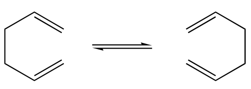 fig. 1: Cope rearrangement.
 -
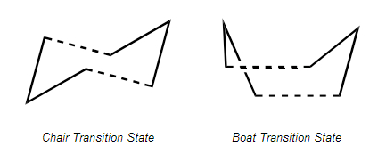 fig.2: Cope rearrangement transition states


At the end of each section in this report, links the log files associated with each calculation will be listed.
Optimising the Reactants and Products
Initially a conformer of hexadiene with an anti-periplanar linkage was optimised using a HF/3-21G basis set:
| File Type | .chk |
|---|---|
| Calculation Type | FOPT |
| Calculation Method | RHF |
| Basis Set | 3-21G |
| Energy (a.u.) | -231.69260226 |
| Gradient (a.u.) | 0.00003016 |
| Dipole Moment (Debye) | 0.2025 |
| Point Group | C2 |
Next, a gauche conformer of the hexadiene was optimised using the same calculation
| File Type | .chk |
|---|---|
| Calculation Type | FOPT |
| Calculation Method | RHF |
| Basis Set | 3-21G |
| Energy (a.u.) | -231.68916011 |
| Gradient (a.u.) | 0.00003227 |
| Dipole Moment (Debye) | 0.5361 |
| Point Group | C0 |
Using appendix A in the script, a conformer called APP2, an anti-periplanar configuration was optimised:
| File Type | .chk |
|---|---|
| Calculation Type | FOPT |
| Calculation Method | RHF |
| Basis Set | 3-21G |
| Energy (a.u.) | -231.69253529 |
| Gradient (a.u.) | 0.00000776 |
| Dipole Moment (Debye) | 0.0001 |
| Point Group | Ci |
The energy value compares favourably with the value given in the appendix (-231.69254), indicating that the correct conformer was optimised. Having identified the conformer it was then optimised further using a larger basis set, namely B3LYP/6-31G*:
| File Type | .chk |
|---|---|
| Calculation Type | FOPT |
| Calculation Method | RB3LYP |
| Basis Set | 6-31G(d) |
| Energy (a.u.) | -234.61171035 |
| Gradient (a.u.) | 0.00001362 |
| Dipole Moment (Debye) | 0.000 |
| Point Group | Ci |
It is clear from the energy value that utilising a larger basis set results in a lower energy and hence a better optimisation. The success of the optimisation was further clarified by running a frequency calculation. The output log file displayed no imaginary frequencies:
 Low frequencies ---   -9.4880    0.0006    0.0008    0.0010    3.7366   13.0029
 Low frequencies ---   74.2857   80.9985  121.4168
In addition to the vibrational information, the frequency analysis also provided a breakdown of energy data under the thermochemistry section of the log file.
 Zero-point correction=                           0.142507 (Hartree/Particle)
 Thermal correction to Energy=                    0.149853
 Thermal correction to Enthalpy=                  0.150797
 Thermal correction to Gibbs Free Energy=         0.110933
 Sum of electronic and zero-point Energies=           -234.469204
 Sum of electronic and thermal Energies=              -234.461857
 Sum of electronic and thermal Enthalpies=            -234.460913
 Sum of electronic and thermal Free Energies=         -234.500777
Log files for calculations in this section:
GAUCHE4 Optimisation (HF/3-21G)
APP2 Optimisation (B3LYP/6-31G*)
Optimising the "Chair" and "Boat" Transition States
Having optimised the reactants and therefore the products of the Cope rearrangement, the next step was to investigate the transition state between them. In this particular reaction, the transition state can take either of two conformations: chair or boat.
Optimising the Chair
The chair conformer was generated in two ways, one using a force constant matrix on a guess of the transition state structure and another where the coordinates of the bonds that are made/broken are fixed before optimisation.
The first method required a guess of the transition state so two allyl fragments were positioned in a shape resembling the chair transition state. An OPT+FREQ calculation was then performed but instead of optimising to a minimum, the structure was optimised to a transition state:
- Optimisation of the chair transition state
-
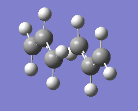 fig. 3: Allyl fragments pre-optimisation.
 -
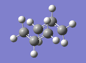 fig. 4: Chair TS after initial optimisation.
 -
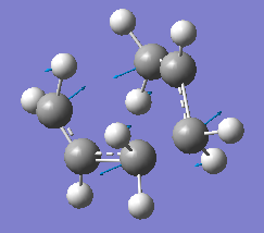 fig. 5: Imaginary vibration which corresponds to the rearrangement.


The resultant interatomic distances along the bonds that are broken/formed were 2.02 A.
The second method involved fixing these interatomic distances while the structure was optimised before then optimising the whole molecule. This was to ensure that the force constant does not need to be calculated, saving time. In this case, the molecule was not complex so the time difference was negligible but for a larger molecule this method can be extremely useful. Firstly the interatomic distances were set at 2.2 A and these bonds were frozen. The rest of the structure was optimised before the bonds were unfrozen to complete the optimisation. The resulting transition state had the same appearance as the first and had interatomic distances of 2.02 A. This shows that in this example, both methods are successful and they also match with the literature value for the computation using the 3-21G basis set which is 2.020 A.[1]
Log Files:
Allyl Fragment Optimisation (HF/3-21G)
Chair Optimisation: Method 1, Method 2 (frozen bonds), Method 2 (Derivatives), Method 2 (B3lYP/6-31G*)
Optimising the Boat
Having generated a model of the chair transition state, the next step was to optimise the boat. This optimisation was undertaken using a completely different method. The optimised structure of APP2 hexadiene was used to represent the reactants and products before a TS(QST2) transition state optimisation was run to identify the transition state between the two. The initial optimisation yielded an unwanted result; a chair transition state was formed:
-
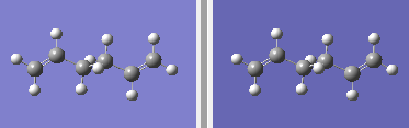 fig. 6: Reactant and product molecules.
 -
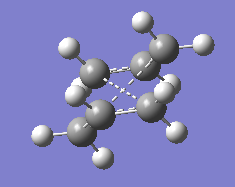 fig. 7: Transition state produced.


The central bond needed to be rotated manually as the computer programme would not consider a rotation when calculating the transition state. The bond was rotated a full 180 degrees and the two C-C-C angles were changed to 100 degrees. The result this time was the boat transition state:
-
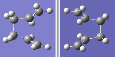 fig. 8: Reactant and product molecules.
 -
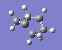 fig. 9: Transition state produced.


Log Files:
Boat optimisation (B3LYP/6-31G*)
Calculating the IRC
Now the tranisition states had been isolated, it was then possible to predict which conformation of hexadiene corresponds to each transition state. This was investigated by calculating the intrinsic reaction coefficients of both the chair and the boat. Force constants were calculated with each step and a limit of 50 steps was applied to each calculation.
Chair IRC
Firstly the IRC of the chair was run. Graphical representation of the reaction progress was obtained from the log file:
-
 graph 1: Chair IRC result. Total energy along the IRC.
 -
 graph 2: Chair IRC result. RMS gradient norm.


It was clear that the energy had tended towards a minimum but the gradient norm was not yet zero. Hence the final step of along the IRC cannot be considered to be the final energy of the product.
Boat IRC
Next the IRC of the boat was run. Graphical representation of the reaction progress was obtained from the log file:
-
 graph 3: Boat IRC result. Total energy along the IRC.
 -
 graph 4: Boat IRC result. RMS gradient norm.


It was clear that again the energy had tended towards a minimum but the gradient norm was not yet zero. In order to discern the conformation of the final products, a further minimisation was required.
Log Files:
Chair IRC Optimised (HF/3-21G)
Discerning the Product Conformation
The final structure of each calculation was optimised to compensate for the incomplete minimisation by the IRC. This could also be done by increasing the number of steps in the IRC calculation but running an optimisation was more time efficient. The final results were as follows:
-
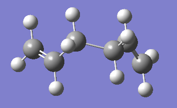 fig. 10: Optimised chair IRC result.
 -
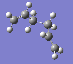 fig. 11: Optimised boat IRC result.


Comparing these structures to those in the Appendix 1, it is clear that the chair transition state tends towards the "Gauche 2" conformer while the boat tends towards the "Gauche 3" conformer. The "Gauche 2" conformer is the lowest energy conformation of all which means that obtaining the lowest energy conformation requires a reaction path through the chair transition state:
| Type of Transition state | Energy of IRC output (a.u.) | Point group of IRC output | Corresponding conformer from Appendix 1 | Energy of conformer in appendix 1 (a.u.) | Point group of conformer in appendix 1 |
|---|---|---|---|---|---|
| Chair | -231.69166702 | C2 | Gauche 2 | -231.69167 | C2 |
| Boat | -231.69266121 | C1 | Gauche 3 | -231.69266 | C1 |
Calculating the Activation Energy
Having determined the reactants for each transition state, the next step was to calculate the activation energy, i.e. the difference in energy beween reactant conformer and transition state. The transition states and reactants were optimised using two different basis sets: HF/3-21G and B3YLP/6-31G* for the purposes of comparison and the although the products may be different, the same reactant was used for the calculation. The reactant chosen was APP2, a conformer already optimised at both levels of theory (All log files have already been linked earlier in the report). The relevant energy values were found in the thermochemistry section of the log file:
| HF/3-21G | B3YLP/6-21G* | |||||
|---|---|---|---|---|---|---|
| Electronic Energy | Sum of Electronic and Zero-Point Energies | Sum of Electronic and Thermal Energies | Electronic Energy | Sum of Electronic and Zero-Point Energies | Sum of Electronic and Thermal Energies | |
| at 0 K | at 298.15 K | at 0 K | at 298.15 K | |||
| Chair TS | -231.619322 | -231.466705 | -231.461345 | -234.556982 | -234.414934 | -234.409011 |
| Boat TS | -231.602802 | -231.450927 | -231.445298 | -234.543093 | -234.402342 | -234.396008 |
| Reactant (APP2) | -231.692535 | -231.539540 | -231.532566 | -234.611710 | -234.469204 | -234.461857 |
| HF/3-21G | B3YLP/6-21G* | Expt. | |||
|---|---|---|---|---|---|
| at 0 K | at 298.15 K | at 0 K | at 298.15 K | at 0 K | |
| ΔE Chair | 45.70 | 44.69 | 34.05 | 33.16 | 33.5 ± 0.5 |
| ΔE Boat | 55.60 | 54.76 | 41.96 | 41.32 | 44.7 ± 2.0 |
What is clear is the use of a large basis set retains the geometry of the molecules in question but has a significant effect on the energies. The activation energies produced by the higher basis set are a lot closer to those expected.
The Diels-Alder Cycloaddition
Introduction
The first section of this investigation demonstrated the various techniques that can be used to analyse a simple organic reaction. The next step was to apply these techniques to a different reaction, namely the Diels-Alder reaction. Again the key to learning about the reaction lay in the transition state with emphasis placed on the HOMO and LUMO as this particular process is pericyclic. Two reactions were studied: ethene with cis-butadiene and maleic anhydride with cyclohexa-1,3-diene.
Optimising the Reactants
Like with the Cope rearrangement, the first stage in producing the transition state was to optimise the reactants. Firstly a molecule of cis-butadiene was constructed on gaussian. This molecule was optimised at the semi-empirical/AM1 level of theory which produced a planar structure. When optimised at a higher level of theory (B3LYP/6-31G*), the dihedral angle was no longer 0 degrees. The structure was bent. For the purposes of this investigation a bent structure is not a useful as studying the MOs is difficult when the symmetry is disrupted. Despite this, the bent structure does conform with structures presented in the literature[2] which cite that the steric hindrance of the terminal CH2 makes a planar structure unfavourable.
-
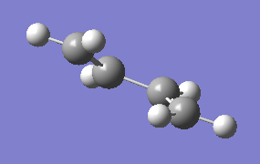 fig. 12: Result of optimisation at B3LYP/6-31G* level.
 -
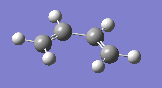 fig. 13: Result of optimisation at semi-empirical/AM1 level.


A molecule of ethene was also optimised and the HOMO/LUMO MOs of each of the reactants were generated:
- Butadiene
-
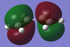 fig. 14: Butadiene HOMO.
 -
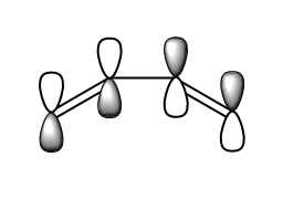 fig. 15: Butadiene HOMO.
 -
 fig. 16: Butadiene LUMO.
 -
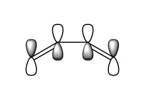 fig. 17: Butadiene LUMO.


Imagining a plane through the central C-C of the molecule, the HOMO is antisymmetric with respect to the plane whist the LUMO is symmetric.
- Ethene
-
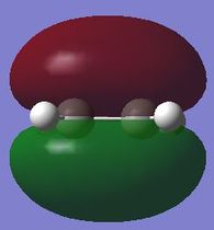 fig. 18: Ethene HOMO.
 -
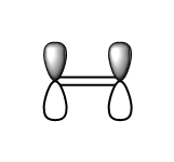 fig. 19: Ethene HOMO.
 -
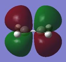 fig. 20: Ethene LUMO.
 -
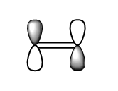 fig. 21: Ethene LUMO.


In contrast with butadiene, the HOMO of ethene is symmetric with respect to the central plane whereas the LUMO is antisymmetric. This implies that the reaction between the two molecules is favourable. Pericyclic reactions are governed by HOMO-LUMO interactions and as the HOMOs both have the same symmetry as the LUMO of the other reactant, there will be lots of favourable HOMO-LUMO interactions in this reaction.
Log Files:
Butadiene Optimisation (B3LYP/6-31G*)
Computing Transition State Geometry
Having optimised the reactants in the Diels-Alder cycloaddition, the next step was to construct the transition state so observe and investigate how the reaction progresses.
Transition State Optimisation
The method chosen for optimisation of the transition state was the frozen coodinate method. The two reactant molecules were superimposed onto one screen in gaussview with the interatomic distances of the bonds to be formed set at 2.20 A. Like in the Cope rearrangement the transition state was optimised with these bonds frozen before the bonds themselves were optimised. The geometry of the resulting transition state was then analysed. The lengths of the sp2 hybridised C-C bonds in the transition state are 1.38 A, slightly higher than the length of a C=C bond in the optimised ethene molecule (and as found in the literature[3]) which are 1.33 A. Sp3 C-C bonds have bond lengths of roughly 1.53 A.[4] This implies that these bonds are in transition between sp2 and sp3 hybridisation. The interatomic distances corresponding to the forming bonds after optimisation were 2.12 A and The Van der Waal's radius of carbon is 1.7 A.[5] Comparing these two figures, it is clear that the carbons are interacting as their VdW radii are overlapping. However, the distance is too great to contitute an sp3 hybridised C-C bond.
The resultant Transition state structure had an imaginary frequency which corresponds to the transition between reactants and products:
-
 fig. 22: Transition state of Diels-Alder Cycloaddition.

This imaginary frequency displayes synchronous bond formation, a key feature of a pericyclic reaction. In contrast, the lowest positive vibration displays some antisynchronous movement. In terms of geometry, the interatomic distance along the two bonds being formed are 2.12 A. Having generated the transition state the HOMO and LUMO were also identified from the calculation:
-
 fig. 23: TS HOMO (anti-symmetric).
 -
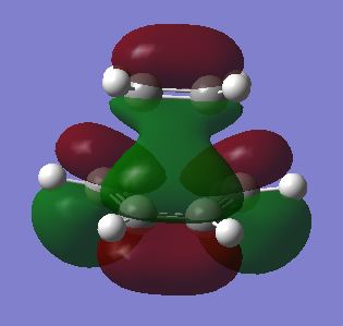 fig. 24: TS LUMO (symmetric).


The HOMO is clearly a mix of the butadiene HOMO and the ethene LUMO which produces an antisymmetric MO. The cycloaddition is allowed because the ethene is behaving as a dienophile and accepting electrons from the HOMO of the electron-rich diene. The symmetry of the corresponding HOMOs and LUMOs are the same which means orbital overlap is significant, a criterion required for an allowed reaction.
Log Files:
Transition State Optimisation (Frozen Bonds) (AM1)
Transition State Optimisation (Derivatives) (AM1)
Transition State IRC
In order to confirm that the transition state generation had indeed been successful, an IRC calculation was run in both directions to analyse the reactants and products. Although the IRC displays a reverse of the cycloaddition, it is still a good method of confirming the transition state:
-
 fig. 25: Reaction movie. Clear transition from reactants to products via a transition state.
 -
 fig. 26: Reaction energy profile.


The reaction energy profile clearly shows reactants, products and an activation energy which needs to be overcome. The top of this peak is the transition state.
Log Files:
Diels-Alder Regioselectivity
Having investigated the simple cycloaddition of cis-butadiene and ethene, the same principles could be used to investigate a different Diels-Alder cycloaddition. The reaction studied was between cyclo-1,3-hexadiene and maleic andhydride. The product of this reaction can take two forms, endo and exo and this regioselectivity was investigated using the methods already used on other molecules and reactions.
Optimising the Reactants and Products
Firstly a molecule of maleic anhydride and a molecule of cyclo-1,3-hexadiene were optimised at the semi-empirical/AM1 level
Log Files:
Cyclohexadiene Optimisation (AM1)
Maleic Anhydride Optimisation (AM1)
Generating Transition States
The next step was to generate the two different transition states: endo and exo. The maleic anhydride was super imposed onto the cyclohexadiene in a way such that the interatomic distances of the forming bonds were 2.2 A. Again, the frozen coordinate method was used to optimise the transition states. This time, the basis set used was HF/3-21G. Each one had an imaginary frequency corresponding to the bond forming reaction:
-
 fig. 27: Imaginary vibration in the endo transition state.
 -
 fig. 28: Imaginary vibration in the exo transition state.


Both transition demonstrate synchronous bond formation in their imaginary frequencies, just like in the cycloaddition of butadiene and ethene. The lowest positive frequency does not contribute to bond forming whatsoever.
The major difference between the two different transition structures is not their behaviour during the reaction but their difference in stability. The energies, geometries and MOs of the exo and endo transition states were analysed to explain any differences.
The energy of each of the transition states was taken from the log files:
| Transition State Conformation | Energy of Optimised TS (a.u.) | Energy of Optimised TS (kJ/mol) |
|---|---|---|
| Endo | -605.61036813 | -1590030 |
| Exo | -605.60359112 | -1590012 |
The energy calculations demonstrate that the endo transition state is lower in energy by ~18 kJ/mol. This means the activation energy for reaction is lower and hence, under kinetic control, the endo product is favoured.
In order to describe the reasons for this stability distance, the geometries and HOMO/LUMOs were analysed and compared. Firstly, the key C-C bond lengths and through space interatomic distances were compared:
-
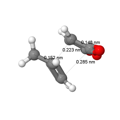 fig. 29: Bond lengths and through space distances for endo transition state.
 -
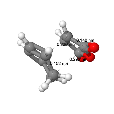 fig. 30: Bond lengths and through space distances for exo transition state.


While the C-C bond lengths on the cyclohexadiene and maleic anhydride are the same on both transition states. However, the through space interactions for the endo transition state are slightly smaller. This implies that the forming bonds are stronger and orbital overlap is better. Sterically this is unexpected as endo structures are more sterically hindered. One reason for this could be down to the bridging group. In the exo transition state the maleic anhydride is in close proximity with a CH2-CH2 group whereas in the endo transition state it is a less bulky CH=CH. This steric repulsion would cause a greater through space difference between the two reactants which destabilises the transition state. The major affect that favours the endo structure however is secondary orbital overlap which can be investigated by constructing the HOMOs and LUMOS.
-
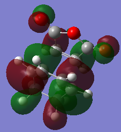 fig. 31: HOMO of endo TS.
 -
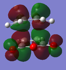 fig. 32: LUMO of endo TS.
 -
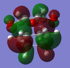 fig. 33: HOMO of exo TS.
 -
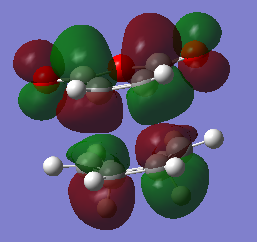 fig. 34: LUMO of exo TS.


In both transition states there is good overlap between the bond forming carbons as expected. These are primary orbital interactions. However, on the endo structure, the C=O bond can also contribute to orbital overlap.
-
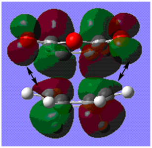 fig. 35: LUMO of endo TS with arrows representing secondary orbital overlap.

Any extra stabilisation due to orbital effects outweighs the unfavourable sterics to make the endo transition state kinetically favoured. In the exo transition state all of the electron density on the diene is positioned on the double bonds so the CO-O-CO fragment cannot engage in any orbital overlap whatsoever.
Log Files:
Endo TS Optimisation (Frozen Bonds)
Endo TS Optimisation (Derivatives)
Exo TS Optimisation (Frozen Bonds)
Endo TS Optimisation (Derivatives)
References
- ↑ K. N. Hod, S. M. Gustafson, & K. A. Black; J. Am. Chem. Soc., Vol. 114, No. 22, 1992
- ↑ Julia E. Rice & Bowen Liu; The Structure of cis-Butadiene; Chemical Physics Letters; 161; 3; 1989; 277–284 DOI:10.1016/S0009-2614(89)87074-5
- ↑ L. S. Bartell1 & R. A. Bonham1; J. Chem. Phys.; 1959; 31; 400. DOI:10.1063/1.1730366
- ↑ Hedberg & Schomaker; J. Am. Chem. Soc.; 1951; 73; 1486.
- ↑ A. Bondi; J. Phys. Chem.; 1964; 68; 441. DOI:10.1021/j100785a001