
Rep:Mod:daw1
Inorganic Computational Lab
Introduction
The modelling of molecular structures using computational methods is a key method of evaluating and predicting the properties of such structures. This investigation demonstrates how these calculations can be made and applied to ionic liquids.
Note on Format of Report
Each calculation is accompanied by its associated output file.
In the cases where the calculation was made on Gaussian on the computer, there is a link to the log file for the computation integrated into either the table caption or the appropriate heading.
Where the calculation has been performed using the HPC, there will be a superscript number in the table caption or heading which links to a D-space file referenced at the end of the section.
Carrying out Simple Calculations on Gaussian
BH3 Manipulation and Optimisation
A molecule of BH3 was constructed on Gaussview 5.0. The bond lengths were augmented to lengths of 1.53A, 1.54A and 1.55A and an optimisation calculation was then run on the molecule to minimise its energy. The resulting molecule had bond lengths of 1.19A. The three bond angles were all 120.0 degrees. One would expect identical bond lengths and angles and the computation was accurate in doing this. Further information can be gleaned from the calculation:
| File Type | .log file |
|---|---|
| Calculation Type | FOPT |
| Calculation Method | RB3LYP |
| Basis Set | 3-21G |
| Final Energy (au) | -26.46226429 |
| Gradient (au) | 0.00008851 |
| Dipole Moment (Debye) | 0.0003 |
| Point Group | Cs |
| Calculation Time (s) | 73.0 |
         Item               Value     Threshold  Converged?
 Maximum Force            0.000220     0.000450     YES
 RMS     Force            0.000106     0.000300     YES
 Maximum Displacement     0.000709     0.001800     YES
 RMS     Displacement     0.000447     0.001200     YES
 Predicted change in Energy=-1.672479D-07
 Optimization completed.
    -- Stationary point found.
                           ----------------------------
                           !   Optimized Parameters   !
                           ! (Angstroms and Degrees)  !
 --------------------------                            --------------------------
 ! Name  Definition              Value          Derivative Info.                !
 --------------------------------------------------------------------------------
 ! R1    R(1,2)                  1.1947         -DE/DX =   -0.0002              !
 ! R2    R(1,3)                  1.1944         -DE/DX =   -0.0001              !
 ! R3    R(1,4)                  1.1948         -DE/DX =   -0.0002              !
 ! A1    A(2,1,3)              119.9983         -DE/DX =    0.0                 !
 ! A2    A(2,1,4)              120.0157         -DE/DX =    0.0                 !
 ! A3    A(3,1,4)              119.986          -DE/DX =    0.0                 !
 ! D1    D(2,1,4,3)            180.0            -DE/DX =    0.0                 !
 --------------------------------------------------------------------------------
 GradGradGradGradGradGradGradGradGradGradGradGradGradGradGradGradGradGrad
The optimisation was then run using a larger basis set, namely 6-31G(d,p):
| File Type | .log file |
|---|---|
| Calculation Type | FOPT |
| Calculation Method | RB3LYP |
| Basis Set | 6-31G(d,p) |
| Final Energy (au) | -26.61532361 |
| Gradient (au) | 0.00000706 |
| Dipole Moment (Debye) | 0.0001 |
| Point Group | Cs |
| Calculation Time (s) | 5.0 |
 Item               Value     Threshold  Converged?
 Maximum Force            0.000204     0.000450     YES
 RMS     Force            0.000099     0.000300     YES
 Maximum Displacement     0.000875     0.001800     YES
 RMS     Displacement     0.000418     0.001200     YES
 Predicted change in Energy=-1.452109D-07
 Optimization completed.
    -- Stationary point found.
                           ----------------------------
                           !   Optimized Parameters   !
                           ! (Angstroms and Degrees)  !
 --------------------------                            --------------------------
 ! Name  Definition              Value          Derivative Info.                !
 --------------------------------------------------------------------------------
 ! R1    R(1,2)                  1.1928         -DE/DX =   -0.0002              !
 ! R2    R(1,3)                  1.1926         -DE/DX =   -0.0002              !
 ! R3    R(1,4)                  1.1924         -DE/DX =    0.0                 !
 ! A1    A(2,1,3)              120.0146         -DE/DX =    0.0                 !
 ! A2    A(2,1,4)              119.9866         -DE/DX =    0.0                 !
 ! A3    A(3,1,4)              119.9988         -DE/DX =    0.0                 !
 ! D1    D(2,1,4,3)            180.0            -DE/DX =    0.0                 !
 --------------------------------------------------------------------------------
 GradGradGradGradGradGradGradGradGradGradGradGradGradGradGradGradGradGrad
Using the larger basis set, the bond lengths were 1.19A, 1.19A and 1.19A and the bond angles were again all 120.0 degrees. The use of a larger basis set meant that the bond lengths were slightly smaller and also had a smaller range when observed beyond two decimal places. However, bond lengths calculated using these methods are not accurate beyond two decimal places and therefore the increased basis set does not necessarily improve the bond length assessment. The bond angles are identical to when the smaller basis set was used (120.0 degrees) which is to be expected for a trigonal planar structure.
Using Pseudo-Potentials and Larger Basis Sets
The next step was to optimise a larger and more energetically complex molecule: GaBr3. This calculation required the HPC supercomputer to be performed and before the calculation was made the symmetry was set to D3h:
| File Type | .log file |
|---|---|
| Calculation Type | FOPT |
| Calculation Method | RB3LYP |
| Basis Set | LANL2DZ |
| Final Energy (au) | -41.70082783 |
| Gradient (au) | 0.00000016 |
| Dipole Moment (Debye) | 0.0000 |
| Point Group | D3H |
| Calculation Time (s) | 13.3 |
       Item               Value     Threshold  Converged?
 Maximum Force            0.000000     0.000450     YES
 RMS     Force            0.000000     0.000300     YES
 Maximum Displacement     0.000003     0.001800     YES
 RMS     Displacement     0.000002     0.001200     YES
 Predicted change in Energy=-1.282691D-12
 Optimization completed.
    -- Stationary point found.
                           ----------------------------
                           !   Optimized Parameters   !
                           ! (Angstroms and Degrees)  !
 --------------------------                            --------------------------
 ! Name  Definition              Value          Derivative Info.                !
 --------------------------------------------------------------------------------
 ! R1    R(1,2)                  2.3502         -DE/DX =    0.0                 !
 ! R2    R(1,3)                  2.3502         -DE/DX =    0.0                 !
 ! R3    R(1,4)                  2.3502         -DE/DX =    0.0                 !
 ! A1    A(2,1,3)              120.0            -DE/DX =    0.0                 !
 ! A2    A(2,1,4)              120.0            -DE/DX =    0.0                 !
 ! A3    A(3,1,4)              120.0            -DE/DX =    0.0                 !
 ! D1    D(2,1,4,3)            180.0            -DE/DX =    0.0                 !
 --------------------------------------------------------------------------------
 GradGradGradGradGradGradGradGradGradGradGradGradGradGradGradGradGradGrad
The bond lengths in this case are all 2.35A. The bond angles are all 120.0 degrees. Setting the symmetry before the calculation was made ensured that these bond lengths and angles were identical in the optimised molecule.
BBr3 was then optimised:
| File Type | .log file |
|---|---|
| Calculation Type | FOPT |
| Calculation Method | RB3LYP |
| Basis Set | Gen |
| Final Energy (au) | -64.43645388 |
| Gradient (au) | 0.00000943 |
| Dipole Moment (Debye) | 0.0005 |
| Point Group | CsH |
| Calculation Time (s) | 24.1 |
        Item               Value     Threshold  Converged?
 Maximum Force            0.000016     0.000450     YES
 RMS     Force            0.000010     0.000300     YES
 Maximum Displacement     0.000067     0.001800     YES
 RMS     Displacement     0.000040     0.001200     YES
 Predicted change in Energy=-1.574159D-09
 Optimization completed.
    -- Stationary point found.
                           ----------------------------
                           !   Optimized Parameters   !
                           ! (Angstroms and Degrees)  !
 --------------------------                            --------------------------
 ! Name  Definition              Value          Derivative Info.                !
 --------------------------------------------------------------------------------
 ! R1    R(1,2)                  1.934          -DE/DX =    0.0                 !
 ! R2    R(1,3)                  1.934          -DE/DX =    0.0                 !
 ! R3    R(1,4)                  1.9339         -DE/DX =    0.0                 !
 ! A1    A(2,1,3)              119.9971         -DE/DX =    0.0                 !
 ! A2    A(2,1,4)              120.0011         -DE/DX =    0.0                 !
 ! A3    A(3,1,4)              120.0018         -DE/DX =    0.0                 !
 ! D1    D(2,1,4,3)            180.0            -DE/DX =    0.0                 !
 --------------------------------------------------------------------------------
 GradGradGradGradGradGradGradGradGradGradGradGradGradGradGradGradGradGrad
In this case, the bond lengths were 1.93A. The bond angles were again all 120 degrees.
Comparing the Structures
| Molecule | Calculated Bond Length (A) | Literature Bond Length (A) |
|---|---|---|
| BH3 | 1.19 | 1.188[3] |
| BBr3 | 1.93 | 1.903[4] |
| GaBr3 | 2.35 | 2.243[5] |
Firstly, the BH3 and BBr3 bond lengths were compared. Changing the ligand from H to Br increases bond length by ~0.74 A which is considerable (62 % of the B-H bond length). The main reason for this is the size of bromine's atomic radius which is much larger than that of hydrogen as it has d and p orbitals. However, the increased electronegativity of bromine means that the B-Br bond is more polar and this strengthens the bond. The bond is slightly shortened because of this but not by enough to overcome the effect of atomic radius.
Comparing the GaBr3 bond lengths and BBr3 bond lengths allowed investigation into how changing the central ion changes them. Like before, there is a marked increase in atomic radius which results in a longer bond in GaBr3 bond. However, the difference in bond length is less pronounced than when the ligand was altered. This could be because gallium and bromine are in the same period of the periodic table. This means that their atomic radii are similar. The result of this is favourable orbital overlap which strengthens the bond and decreases its length. Again however this effect is not strong enough to overcome the overall effect of the larger atomic radius of gallium.
Overall, the bond lengths match fairly well with the literature, indicating that the computational methods can provide an acceptable estimate of bond length. However, more accuracy is required to match the literature to the same accuracy and precision.
When analysing molecules in gaussview, the image of the molecule displays the bonds as well as position of the atoms. However, if a calculation results in a bond length with a magnitude above a certain distance the bond disappears. Gaussview has an objective measure of what is or isn't a bond based on numbers, in this case the bond length. However, actually defining what what a bond is requires more subtlety and subjectivity. If the electronic interaction between two atoms is sufficient to consider the two to be one system and highly dependent on each other then, regardless of distance they are a bond. However, bond distance can be a very good indicator of bond strength and therefore above a certain bond length said bond may be very weak indeed.
References for this Section
- ↑ Dominic Wood, D-Space, 2013 DOI:10042/26104
- ↑ Dominic Wood, D-Space, 2013 DOI:10042/26196
- ↑ B. Ruščić, C. A. Mayhew and J. Berkowitz; "Photoionization studies of (BH3) n (n=1,2)"; J. Chem. Phys.; 1988; 88; 5580 DOI:10.1063/1.454569
- ↑ G. Santiso-Quiñones Dr., I. Krossing Prof. Dr.; "Reference Values for the B-X Bond Lengths of BI3 and BBr3"; ZAAC; 2008; 634; 704-707 DOI:10.1002/zaac.200700510
- ↑ B. K. Ystenesa, M. Ystenes and G. Scholz; "Ab initio quantum mechanical vibrational analysis of planar AX3 molecules (A is Al, Ga, In; X is F, Cl, Br, I)"; Spectrochimica Acta Part A: Molecular and Biomolecular Spectroscopy; 1995; 51; 2481–2489 DOI:10.1016/0584-8539(95)01483-7
More Complex Analysis
BH3 Frequency Analysis
The BH3 optimisation result was used to conduct frequency analysis to investigate the vibrations of the molecule. When running the frequency computation, the same basis set as the optimisation (6-31G (d,p) in the case of BH3) is used along with the same method. This is important as the calculation is a continuation of the optimisation and therefore the frequency analysis calculation would not recognise the optimised structure as the low energy form were a different mode or basis set used. Frequency analysis is carried out to investigate vibrations about an equilibrium with the equilibrium being the optimised structure so in order for it to be a success, the optimised structure must be the same throughout. The result of a frequency analysis calculation is a set of frequencies which correspond to 3N-6 vibrational modes. The "-6" represents movement of the centre of mass of the molecule and hence should have a value of very close to zero. In order to verify the success of a frequency analysis computation the values of these "zero frequencies" should be as close to zero as possible (usually within +/- 15.0 cm-1):
| File Type | .log file |
|---|---|
| Calculation Type | FREQ |
| Calculation Method | RB3LYP |
| Basis Set | 6-31G(d,p) |
| Final Energy (au) | -26.61532363 |
| Gradient (au) | 0.00000286 |
| Dipole Moment (Debye) | 0.0000 |
| Point Group | D3H |
| Calculation Time (s) | 4.0 |
        Item               Value     Threshold  Converged?
 Maximum Force            0.000006     0.000450     YES
 RMS     Force            0.000003     0.000300     YES
 Maximum Displacement     0.000022     0.001800     YES
 RMS     Displacement     0.000011     0.001200     YES
 Predicted change in Energy=-1.923583D-10
 Optimization completed.
    -- Stationary point found.
 GradGradGradGradGradGradGradGradGradGradGradGradGradGradGradGradGradGrad
Low frequencies ---   -0.9390   -0.8456   -0.0054    5.8509   11.7777   11.8151
 Low frequencies --- 1162.9967 1213.1829 1213.1856
 Diagonal vibrational polarizability:
        0.7181156       0.7180154       1.8413830
 Harmonic frequencies (cm**-1), IR intensities (KM/Mole), Raman scattering
 activities (A**4/AMU), depolarization ratios for plane and unpolarized
 incident light, reduced masses (AMU), force constants (mDyne/A),
 and normal coordinates:
                      1                      2                      3
                     A2"                    E'                     E'
 Frequencies --   1162.9967              1213.1829              1213.1856
 Red. masses --      1.2531                 1.1072                 1.1072
 Frc consts  --      0.9986                 0.9601                 0.9601
 IR Inten    --     92.5482                14.0551                14.0588
  Atom  AN      X      Y      Z        X      Y      Z        X      Y      Z
     1   5     0.00   0.00   0.16     0.00   0.10   0.00    -0.10   0.00   0.00
     2   1     0.00   0.00  -0.57     0.00   0.08   0.00     0.81   0.00   0.00
     3   1     0.00   0.00  -0.57    -0.39  -0.59   0.00     0.14   0.39   0.00
     4   1     0.00   0.00  -0.57     0.39  -0.59   0.00     0.14  -0.39   0.00
The low frequency values shown above indicate that the frequency analysis has been successful as the largest of the "zero frequencies" is less than 15 cm-1 and the other low frequencies are positive and large.
The vibrations were then analysed on Gaussview:
| Vibration Mode Number | Vibration Image | Vibration Frequency | Infrared | Symmetry (D3h point group) | Description |
|---|---|---|---|---|---|
| 1 | 
|
1163 | 93 | A2 | All 3 hydrogens perform a wagging motion in and out of plane with the stationary boron. |
| 2 | 
|
1213 | 14 | E' | Two of the hydrogens perform a scissoring action while the boron and other hydrogen are effectively stationary disregarding slight recoil motion. |
| 3 | 
|
1213 | 14 | E' | Two hydrogens perform a rocking motion while the other bends with greater magnitude in the same plane. The boron is stationary. |
| 4 | 
|
2582 | 0 | A1' | Concerted symmetric stretch of the three hydrogens away from the stationary boron. |
| 5 | 
|
2715 | 126 | E' | Two of the hydrogens undergo asymmetric stretching while the boron and other hydrogen remain stationary. |
| 6 | 
|
2715 | 126 | E' | Two hydrogens undergo symmetric stretching. The other stretches with greater magnitude asymmetrically with respect to the other hydrogens. The boron is stationary. |
These vibrational modes are displayed in graphical form on an infrared spectrum:

Although there are 6 vibrations, there are two pairs of vibrations which have very similar frequencies (2 & 3 and 5 & 6). These signals overlap in the spectrum. In addition, vibrational mode 4 does not have a change of dipole moment and hence does not appear in the IR spectrum.
GaBr3 Frequency Analysis
The same analysis was carried out on a molecule of GaBr3:
| File Type | .log file |
|---|---|
| Calculation Type | FREQ |
| Calculation Method | RB3LYP |
| Basis Set | LANL2DZ |
| Final Energy (au) | -41.70082783 |
| Gradient (au) | 0.00000011 |
| Dipole Moment (Debye) | 0.0000 |
| Point Group | D3H |
| Calculation Time (s) | 8.3 |
       Item               Value     Threshold  Converged?
 Maximum Force            0.000000     0.000450     YES
 RMS     Force            0.000000     0.000300     YES
 Maximum Displacement     0.000002     0.001800     YES
 RMS     Displacement     0.000001     0.001200     YES
 Predicted change in Energy=-6.142863D-13
 Optimization completed.
    -- Stationary point found.
 GradGradGradGradGradGradGradGradGradGradGradGradGradGradGradGradGradGrad
 Low frequencies ---   -0.5252   -0.5247   -0.0024   -0.0010    0.0235    1.2010
 Low frequencies ---   76.3744   76.3753   99.6982
 Diagonal vibrational polarizability:
       30.7937168      30.7942540      24.9520712
 Harmonic frequencies (cm**-1), IR intensities (KM/Mole), Raman scattering
 activities (A**4/AMU), depolarization ratios for plane and unpolarized
 incident light, reduced masses (AMU), force constants (mDyne/A),
 and normal coordinates:
                      1                      2                      3
                     E'                     E'                     A2"
 Frequencies --     76.3744                76.3753                99.6982
 Red. masses --     77.4211                77.4212                70.9513
 Frc consts  --      0.2661                 0.2661                 0.4155
 IR Inten    --      3.3447                 3.3447                 9.2161
  Atom  AN      X      Y      Z        X      Y      Z        X      Y      Z
     1  31    -0.39   0.00   0.00     0.00   0.39   0.00     0.00   0.00   0.89
     2  35     0.63   0.00   0.00     0.00   0.41   0.00     0.00   0.00  -0.26
     3  35    -0.15  -0.45   0.00     0.45  -0.37   0.00     0.00   0.00  -0.26
     4  35    -0.15   0.45   0.00    -0.45  -0.37   0.00     0.00   0.00  -0.26
                      4                      5                      6
                     A1'                    E'                     E'
 Frequencies --    197.3371               316.1825               316.1863
 Red. masses --     78.9183                72.2067                72.2066
 Frc consts  --      1.8107                 4.2531                 4.2532
 IR Inten    --      0.0000                57.0704                57.0746
  Atom  AN      X      Y      Z        X      Y      Z        X      Y      Z
     1  31     0.00   0.00   0.00     0.82   0.00   0.00     0.00   0.82   0.00
     2  35     0.00   0.58   0.00    -0.01   0.00   0.00     0.00  -0.47   0.00
     3  35    -0.50  -0.29   0.00    -0.35  -0.20   0.00    -0.20  -0.12   0.00
     4  35     0.50  -0.29   0.00    -0.35   0.20   0.00     0.20  -0.12   0.00
Again, Gaussview was used to analyse the vibrations:
| Vibration Mode Number | Vibration Image | Vibration Frequency | Infrared | Symmetry (D3h point group) | Description |
|---|---|---|---|---|---|
| 1 | 
|
76 | 3 | E' | Two bromines undergo a rocking motion while the other bends in the same plane with greater magnitude. The gallium undergoes a little recoil motion |
| 2 | 
|
76 | 3 | E' | Two of the bromines undergo a scisorring motion. The gallium and other bromine move together oscillate slightly due to recoil. |
| 3 | 
|
100 | 9 | A2 | The three bromines undergo a wagging motion with respect to the gallium which undergoes a large oscillatory motion in the opposite direction. |
| 4 | 
|
197 | 0 | A1' | The three bromines undergo symmetric stretching away from the stationary gallium. |
| 5 | 
|
316 | 57 | E' | Two bromines undergo asymmetric stretching causing recoil in the gallium. The other bromine is stationary. |
| 6 | 
|
316 | 57 | E' | Two bromines undergo symmetric stretching while the other stretches anti-symmetrically with respect to the other two. |
An IR spectrum was produced from this calculation:

Comparing the Frequency Analyses of BH3 and GaBr3
| Vibration Number | BH3 frequency (cm-1) | GaBr3 frequency (cm-1) |
|---|---|---|
| 1 | 1163 | 76 |
| 2 | 1213 | 76 |
| 3 | 1213 | 100 |
| 4 | 2582 | 197 |
| 5 | 2715 | 316 |
| 6 | 2715 | 316 |
The frequencies corresponding to the vibrations in the case of GaBr3 are far lower that those in BH3. The increased mass of both central element and ligand are major contributors to this. A lower IR frequency implies the vibrations are of lower energy. This makes sense as, modelling the bonds as springs, frequency is inversely proportional to the square root of the reduced mass of the system. Hence increasing the reduced mass will decrease the frequency.
The vibrational modes involved are slightly re-ordered. The A2 mode is the lowest frequency vibration in BH3 whereas it is the 3rd lowest in GaBr3.
Looking at the two spectra, they have the same pattern of 3 low frequency vibrations (2 degenerate), one vibration missing due to its lack of dipole moment and two degenerate vibrational modes of much higher frequency. This is to be expected as although the masses are different, the structure is the same and therefore the vibrations should follow the same pattern relatively. The large gap in frequency between the lower three modes and the higher three is due to the nature of the vibrations. The lower frequency modes have more bending character whereas the upper three are stretches. Just as in organic IR spectroscopy the bending modes tend to be lower in energy and hence have a lower frequency.
BH3 MO Analysis
The optimised BH3 structure was used to set up a calcutation which would enable analysis of the molecular orbitals of BH3:
| File Type | .log file |
|---|---|
| Calculation Type | SP |
| Calculation Method | RB3LYP |
| Basis Set | 6-31G(d,p) |
| Final Energy (au) | -26.61532361 |
| Gradient (au) | N/A |
| Dipole Moment (Debye) | 0.0001 |
| Point Group | Cs |
| Calculation Time (s) | 7.3 |
The calculated MOs were then compared with the LCAOs which are displayed on an MO diagram

It is clear that in general, the computed MOs fit very well with the theoretically produced LCAOs. This is evidence that LCAO MO theory is a useful tool for predicting molecular orbitals. However, only the vague shape matches. Particularly for more complex MOs, an accurate shape is produced better using the computational method. LCAO theory is only qualitative and although it has been shown to be a good visual approximation, it could not be used to investigate the true nature of the MOs.
NH3 NBO Analysis
Firstly a molecule of NH3 was optimised:
| File Type | .log file |
|---|---|
| Calculation Type | FOPT |
| Calculation Method | RB3LYP |
| Basis Set | 6-31G(d,p) |
| Final Energy (au) | -56.55776863 |
| Gradient (au) | 0.00000289 |
| Dipole Moment (Debye) | 1.8464 |
| Point Group | C3V |
| Calculation Time (s) | 14.0 |
        Item               Value     Threshold  Converged?
 Maximum Force            0.000000     0.000450     YES
 RMS     Force            0.000000     0.000300     YES
 Maximum Displacement     0.000002     0.001800     YES
 RMS     Displacement     0.000001     0.001200     YES
 Predicted change in Energy=-6.142863D-13
 Optimization completed.
    -- Stationary point found.
 GradGradGradGradGradGradGradGradGradGradGradGradGradGradGradGradGradGrad
A frequency analysis was then undertaken to check if a minimum energy configuration had been obtained:
| File Type | .log file |
|---|---|
| Calculation Type | FREQ |
| Calculation Method | RB3LYP |
| Basis Set | 6-31G(d,p) |
| Final Energy (au) | -56.55776856 |
| Gradient (au) | 0.00000279 |
| Dipole Moment (Debye) | 1.8464 |
| Point Group | C3 |
| Calculation Time (s) | 8.0 |
         Item               Value     Threshold  Converged?
 Maximum Force            0.000004     0.000450     YES
 RMS     Force            0.000002     0.000300     YES
 Maximum Displacement     0.000038     0.001800     YES
 RMS     Displacement     0.000017     0.001200     YES
 Predicted change in Energy=-1.856666D-10
 Optimization completed.
    -- Stationary point found.
 GradGradGradGradGradGradGradGradGradGradGradGradGradGradGradGradGradGrad
 Low frequencies ---   -7.1411   -2.7552   -0.0005   -0.0004    0.0006    2.9474
 Low frequencies --- 1089.2688 1693.9201 1693.9230
 Diagonal vibrational polarizability:
        0.1277306       0.1277323       3.3014166
 Harmonic frequencies (cm**-1), IR intensities (KM/Mole), Raman scattering
 activities (A**4/AMU), depolarization ratios for plane and unpolarized
 incident light, reduced masses (AMU), force constants (mDyne/A),
 and normal coordinates:
                      1                      2                      3
                      A                      A                      A
 Frequencies --   1089.2688              1693.9201              1693.9230
 Red. masses --      1.1800                 1.0644                 1.0644
 Frc consts  --      0.8249                 1.7995                 1.7995
 IR Inten    --    145.4536                13.5593                13.5592
  Atom  AN      X      Y      Z        X      Y      Z        X      Y      Z
     1   7     0.00   0.00   0.12     0.00   0.07   0.00    -0.07   0.00   0.00
     2   1     0.00  -0.21  -0.53     0.00   0.15   0.26     0.76   0.00   0.00
     3   1     0.18   0.11  -0.53     0.39  -0.53  -0.13     0.08  -0.39   0.22
     4   1    -0.18   0.11  -0.53    -0.39  -0.53  -0.13     0.08   0.39  -0.22
                      4                      5                      6
                      A                      A                      A
 Frequencies --   3461.3599              3589.9198              3589.9345
 Red. masses --      1.0272                 1.0883                 1.0883
 Frc consts  --      7.2512                 8.2639                 8.2640
 IR Inten    --      1.0585                 0.2692                 0.2693
  Atom  AN      X      Y      Z        X      Y      Z        X      Y      Z
     1   7     0.00   0.00   0.04     0.00   0.08   0.00     0.08   0.00   0.00
     2   1     0.00   0.55  -0.18     0.00  -0.75   0.31     0.02   0.00   0.00
     3   1    -0.47  -0.27  -0.18    -0.34  -0.17  -0.15    -0.56  -0.34  -0.27
     4   1     0.47  -0.27  -0.18     0.34  -0.17  -0.15    -0.56   0.34   0.27
A population analysis of NH3 was then carried out:
| File Type | .log file |
|---|---|
| Calculation Type | SP |
| Calculation Method | RB3LYP |
| Basis Set | 6-31G(d,p) |
| Final Energy (au) | -56.55776872 |
| Gradient (au) | 0.00000279 |
| Dipole Moment (Debye) | 1.8464 |
| Point Group | C3 |
| Calculation Time (s) | 5.0 |
Using the .log output from this calculation, a picture of the NBO charge distribution was produced:


As expected, the electronegative nitrogen has a large negative charge compared to the small positive charges on the charges on the hydrogens. The overall charge is 0 as NH3 is a neutral species.
Association Energy of Ammonia-Borane
At this stage only single molecules had been analysed. The next stage was to analyse a reaction, namely the formation of ammonia-borane. The energies of ammonia and borane had already been calculated but the final product had to be analysed computationally. Firstly an optimisation of ammonia-borane was run. In order to obtain the required negative frequencies, the keywords "opt=tight", "nosymm" "int=ultrafine scf=conver=9" were added to the calculation. Therefore new optimisations of BH3 and NH3 were run withe these keywords added:
| NH3BH3 Optimisation | BH3 Optimisation | NH3 Optimisation | |
|---|---|---|---|
| File Type | .log file | .log file | .log file |
| Calculation Type | FOPT | FOPT | FOPT |
| Calculation Method | RB3LYP | RB3LYP | RB3LYP |
| Basis Set | 6-31G(d,p) | 6-31G(d,p) | 6-31G(d,p) |
| Final Energy (au) | -83.22468911 | -26.61532360 | -56.55776872 |
| Gradient (au) | 0.00000125 | 0.00000594 | 0.00000190 |
| Dipole Moment (Debye) | 5.5647 | 0.0001 | 1.8464 |
| Point Group | C1 | Cs | Cs |
| Calculation Time (s) | 94.0 | 8.0 | 5.0 |
NH3BH3:
        Item               Value     Threshold  Converged?
 Maximum Force            0.000002     0.000015     YES
 RMS     Force            0.000001     0.000010     YES
 Maximum Displacement     0.000023     0.000060     YES
 RMS     Displacement     0.000010     0.000040     YES
 Predicted change in Energy=-8.987776D-11
 Optimization completed.
    -- Stationary point found.
BH3
        Item               Value     Threshold  Converged?
 Maximum Force            0.000009     0.000015     YES
 RMS     Force            0.000007     0.000010     YES
 Maximum Displacement     0.000053     0.000060     YES
 RMS     Displacement     0.000034     0.000040     YES
 Predicted change in Energy=-7.783630D-10
 Optimization completed.
    -- Stationary point found.
NH3
        Item               Value     Threshold  Converged?
 Maximum Force            0.000003     0.000015     YES
 RMS     Force            0.000002     0.000010     YES
 Maximum Displacement     0.000026     0.000060     YES
 RMS     Displacement     0.000017     0.000040     YES
 Predicted change in Energy=-1.462193D-10
 Optimization completed.
    -- Stationary point found.
After successful optimisation was achieved, a frequency analysis calculation was carried out to ensure the low frequencies were not too high:
| File Type | .log file |
|---|---|
| Calculation Type | FREQ |
| Calculation Method | RB3LYP |
| Basis Set | 6-31G(d,p) |
| Final Energy (au) | -83.22468911 |
| Gradient (au) | 0.00000121 |
| Dipole Moment (Debye) | 5.5647 |
| Point Group | C1 |
| Calculation Time (s) | 53.0 |
 Low frequencies ---   -3.2461   -2.7380    0.0007    0.0012    0.0014    3.7015
 Low frequencies ---  263.3390  632.9624  638.4407
The energies of reactants and products were then compared:
| Molecule | Molecule Energy (au) |
|---|---|
| NH3 | -26.61532360 |
| BH3 | -56.55776872 |
| NH3BH3 | -83.22468911 |
The energy difference produced by these figures is -0.05159691 au which is -135.467661 kJ/mol. Therefore the bond dissociation energy for the breaking of the B-N bond is ~135.5 kJ/mol. This figure is in to the correct power of ten but is under half the literature value of ~385.0 kJ/mol.[3] However, this literature value is for just a B-N bond and can only be used in order to verify a ballpark figure, which it does.
References for this Section
- ↑ Dominic Wood, D-Space, 2013 DOI:10042/26197
- ↑ Dominic Wood, D-Space, 2013 DOI:10042/26198
- ↑ H. B. Gray; "Chemical bonds: an introduction to atomic and molecular structure"; University Science Books; 1994; 96
Mini-Project - Ionic Liquids: Designer Solvents
Introduction
The first section of this investigation was an introduction to using computational methods to compare different structures and compounds. The next step was to apply this understanding in a more realistic scenario. Ionic liquids have wide ranging properties and by choosing the correct combination of anion and cation it is possible to engineer the desired properties into the solvent. One way to predict these properties without testing in a lab is through computational methods. The key aim of this section was to use the methods already used to analyse a series of different cations for use in these "designer solvents".
All calculations in this project were performed using the same basis set: 6-31G(d,p). In addition to this, the extra keywords "nosymm" and "int=ultrafine scf=conver=9" were added to refine the basis set.
Part I: Comparison of Selected Onium Ions
Optimisation and Frequency Calculations
Initially, optimisations were carried out along with frequency analysis to check if the optimisations were successful.
[N(CH3)4]+ was optimised first:
| File Type | .log file |
|---|---|
| Calculation Type | FOPT |
| Calculation Method | RB3LYP |
| Basis Set | 6-31G(d,p) |
| Final Energy (au) | -214.18127313 |
| Gradient (au) | 0.00004483 |
| Dipole Moment (Debye) | 8.2963 |
| Point Group | C1 |
| Calculation Time (s) | 241.0 |
         Item               Value     Threshold  Converged?
 Maximum Force            0.000068     0.000450     YES
 RMS     Force            0.000027     0.000300     YES
 Maximum Displacement     0.000355     0.001800     YES
 RMS     Displacement     0.000098     0.001200     YES
 Predicted change in Energy=-8.994975D-08
 Optimization completed.
    -- Stationary point found.
The frequency calculation was then carried out:
| File Type | .log file |
|---|---|
| Calculation Type | FREQ |
| Calculation Method | RB3LYP |
| Basis Set | 6-31G(d,p) |
| Final Energy (au) | -214.18127313 |
| Gradient (au) | 0.00004480 |
| Dipole Moment (Debye) | 8.2963 |
| Point Group | C1 |
| Calculation Time (s) | 578.0 |
 Low frequencies ---   -0.0005   -0.0004   -0.0003    5.1865    7.2317    8.4713
 Low frequencies ---  186.0696  289.8543  290.3563
These low frequency values indicate a successful optimisation.
The next cation to be optimised was [P(CH3)4]+:
| File Type | .log file |
|---|---|
| Calculation Type | FOPT |
| Calculation Method | RB3LYP |
| Basis Set | 6-31G(d,p) |
| Final Energy (au) | -500.82701146 |
| Gradient (au) | 0.00002925 |
| Dipole Moment (Debye) | 8.2964 |
| Point Group | C1 |
| Calculation Time (s) | 750.7 |
         Item               Value     Threshold  Converged?
 Maximum Force            0.000162     0.000450     YES
 RMS     Force            0.000037     0.000300     YES
 Maximum Displacement     0.000840     0.001800     YES
 RMS     Displacement     0.000357     0.001200     YES
 Predicted change in Energy=-2.332033D-07
 Optimization completed.
    -- Stationary point found.
Again, frequency analysis was performed to assess the success of the optimisation:
| File Type | .log file |
|---|---|
| Calculation Type | FREQ |
| Calculation Method | RB3LYP |
| Basis Set | 6-31G(d,p) |
| Final Energy (au) | -500.82701146 |
| Gradient (au) | 0.00002922 |
| Dipole Moment (Debye) | 8.2964 |
| Point Group | C1 |
| Calculation Time (s) | 1024.5 |
 Low frequencies ---   -9.3513   -7.3538   -4.7726   -0.0028   -0.0026   -0.0017
 Low frequencies ---  156.3060  192.0171  192.2454
These low frequency values indicated that the optimisation was a success.
Finally, an [S(CH3)3]+ cation was optimised:
| File Type | .log file |
|---|---|
| Calculation Type | FOPT |
| Calculation Method | RB3LYP |
| Basis Set | 6-31G(d,p) |
| Final Energy (au) | -517.68327460 |
| Gradient (au) | 0.00000958 |
| Dipole Moment (Debye) | 4.0984 |
| Point Group | C1 |
| Calculation Time (s) | 1201.1 |
         Item               Value     Threshold  Converged?
 Maximum Force            0.000020     0.000450     YES
 RMS     Force            0.000006     0.000300     YES
 Maximum Displacement     0.001021     0.001800     YES
 RMS     Displacement     0.000334     0.001200     YES
 Predicted change in Energy=-1.272435D-08
 Optimization completed.
    -- Stationary point found.
| File Type | .log file |
|---|---|
| Calculation Type | FREQ |
| Calculation Method | RB3LYP |
| Basis Set | 6-31G(d,p) |
| Final Energy (au) | -517.68327460 |
| Gradient (au) | 0.00000952 |
| Dipole Moment (Debye) | 4.0984 |
| Point Group | C1 |
| Calculation Time (s) | 519.0 |
 Low frequencies ---   -6.3604   -0.0022    0.0052    0.0055    3.1624    8.5766
 Low frequencies ---  162.2162  199.8433  200.2329
Again, the optimisation was proved to be a success.
Cation Geometry Comparison
Having optimised the geometries of the three different cations, the next step was to compare them with each other. Firstly, the bond lengths were compared:
| C-N/C-P/C-S Bond Length (A) | |||
|---|---|---|---|
| [N(CH3)4]+ | [P(CH3)4]+ | [S(CH3)3]+ | |
| Computed Value | 1.51 | 1.82 | 1.82 |
| Literature Value | 1.457-1.492[5] | 1.826[6] | 1.785 - 1.805[7] |
As expected, the N-C bond is the shortest. Nitrogen has the smallest atomic radius and in addition, being in the same period as carbon means that orbital overlap, particularly p-p interaction, is favourable. This strengthens and therefore shortens the C-N bonds. The C-P and C-S bonds are similar in length due to the similarities in the ionic radius of P and S. Their electronegativities are also similar meaning the bond strengths will be alike.
NBO and MO Energy Computations
In order to investigate the cations further, an energy calculation was run on each of the cations:
| [N(CH3)4]+ | [P(CH3)4]+ | [S(CH3)3]+ | |
|---|---|---|---|
| File Type | .log file | .log file | .log file |
| Calculation Type | SP | SP | SP |
| Method | RB3LYP | RB3LYP | RB3LYP |
| Basis Set | 6-31G(d,p) | 6-31G(d,p) | 6-31G(d,p) |
| Energy (au) | -214.18127313 | -500.82701146 | -517.68327460 |
| Gradient | N/A | N/A | N/A |
| Dipole Moment (Debye) | 8.2963 | 8.2964 | 4.0984 |
| Point Group | C1 | C1 | C1 |
| Calculation Time (s) | 55.0 | 57.0 | 34.0 |
Molecular Orbital Analysis
The energy calculation for [N(CH34]+ was used to produce images of the occupied molecular orbitals. Five orbitals were chosen for comment:
- 5 occupied non core MOs in order of increasing energy
-
 fig. 6: MO 1
 -
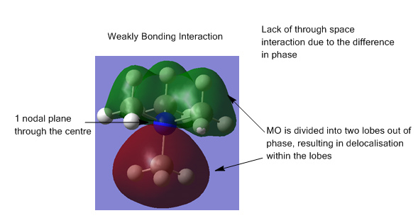 fig. 7: MO 2
 -
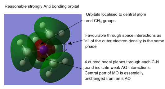 fig. 8: MO 3
 -
 fig. 9: MO 4
 -
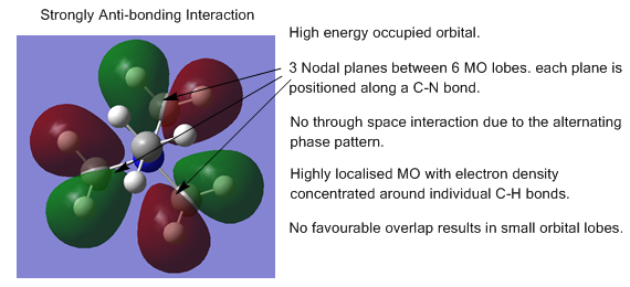 fig. 10: MO 5


In general, the orbitals are quite delocalised with the MOs covering multiple atoms and bonds.
NBO Analysis
The output from the energy calculation was used to analyse the charge distribution across the cations. Each cation carried the same overall charge but the effect of the central element on where this charge is located could be observed from the NBO calculation:
- Charge distribution images from NBO calculation. Charge range = -1.668 to +1.668.
-
![fig. 11: NBO charge distribution of [N(CH3)4]+.](/images/d/d8/DW_COLOURNBO_NCH34.PNG) fig. 11: NBO charge distribution of [N(CH3)4]+.
fig. 11: NBO charge distribution of [N(CH3)4]+. -
![fig. 12: NBO charge distribution of [P(CH3)4]+.](/images/3/36/DW_COLOURNBO_PCH34.PNG) fig. 12: NBO charge distribution of [P(CH3)4]+.
fig. 12: NBO charge distribution of [P(CH3)4]+. -
![fig. 13: NBO charge distribution of [S(CH3)3]+.](/images/8/82/DW_COLOURNBO_SCH33.PNG) fig. 13: NBO charge distribution of [S(CH3)3]+.
fig. 13: NBO charge distribution of [S(CH3)3]+.
![fig. 11: NBO charge distribution of [N(CH3)4]+.](/wiki/File:DW_COLOURNBO_NCH34.PNG)
![fig. 12: NBO charge distribution of [P(CH3)4]+.](/wiki/File:DW_COLOURNBO_PCH34.PNG)
![fig. 13: NBO charge distribution of [S(CH3)3]+.](/wiki/File:DW_COLOURNBO_SCH33.PNG)
- Charge distribution images from NBO calculation with numbered charges. Charge range = -1.668 to +1.668.
-
![fig. 14: NBO charge distribution of [N(CH3)4]+.](/images/thumb/b/b5/DW_NUMBERSNBO_NCH34.PNG/418px-DW_NUMBERSNBO_NCH34.PNG) fig. 14: NBO charge distribution of [N(CH3)4]+.
fig. 14: NBO charge distribution of [N(CH3)4]+. -
![fig. 15: NBO charge distribution of [P(CH3)4]+.](/images/f/f8/DW_NUMBERSNBO_PCH34.PNG) fig. 15: NBO charge distribution of [P(CH3)4]+.
fig. 15: NBO charge distribution of [P(CH3)4]+. -
![fig. 16: NBO charge distribution of [S(CH3)3]+.](/images/b/ba/DW_NUMBERSNBO_SCH33.PNG) fig. 16: NBO charge distribution of [S(CH3)3]+.
fig. 16: NBO charge distribution of [S(CH3)3]+.
![fig. 14: NBO charge distribution of [N(CH3)4]+.](/wiki/File:DW_NUMBERSNBO_NCH34.PNG)
![fig. 15: NBO charge distribution of [P(CH3)4]+.](/wiki/File:DW_NUMBERSNBO_PCH34.PNG)
![fig. 16: NBO charge distribution of [S(CH3)3]+.](/wiki/File:DW_NUMBERSNBO_SCH33.PNG)
| Cation | Central Atom Charge | Carbon Charge | Hydrogen Charge |
|---|---|---|---|
| [N(CH3)4]+ | -0.295 | -0.483 | +0.269 |
| [P(CH3)4]+ | +1.668 | -1.060 | +0.298 |
| [S(CH3)3]+ | +0.917 | -0.846 | +0.297 |
Observing the central atom charges first, it is clear that the electronegativity of the nitrogen means that it carries more negative charge than either S or P. Overall, the magnitudes of the charges in the N cation are lower than those in the other cations. This is due to good orbital overlap between C and N (as a result of having the same valence AOs). These favourable reactions result in the delocalised MOs seen in the previous section of the report. The charge becomes more evenly spread and therefore the charges are of lower magnitude. In general the charge magnitudes of the hydrogens is pretty much independent of the central atom.
The charges with the largest magnitude are on the atoms of the phosphonium cation. Poor atomic overlap combined with having the lowest electronegativity results in localised charge.
The sulphur cation is only 3 coordinated so the charge magnitudes are decreased. There are fewer carbons to withdraw electron density from the sulphur.
As well as charge distribution, the output from the energy computation explains the contribution from each atom towards the formation of the bond. The contributions towards the C-X bonds (X=N/P/S) were found in the respective log files:
X=N;
    (Occupancy)   Bond orbital/ Coefficients/ Hybrids
 ---------------------------------------------------------------------------------
     1. (1.98451) BD ( 1) N   1 - C   2
                ( 66.35%)   0.8146* N   1 s( 25.00%)p 3.00( 74.97%)d 0.00(  0.03%)
                                            0.0000 -0.5000  0.0007  0.0000 -0.2887
                                            0.0000  0.8163 -0.0001  0.0000  0.0000
                                            0.0097  0.0000  0.0000  0.0120  0.0089
                ( 33.65%)   0.5801* C   2 s( 20.78%)p 3.80( 79.05%)d 0.01(  0.16%)
                                           -0.0003 -0.4552  0.0237 -0.0026  0.2962
                                            0.0126 -0.8375 -0.0356  0.0000  0.0000
                                            0.0221  0.0000  0.0000  0.0273  0.0203
X=P:
  4. (1.98032) BD ( 1) C   1 - P  17
                ( 59.58%)   0.7719* C   1 s( 25.25%)p 2.96( 74.66%)d 0.00(  0.08%)
                                            0.0002  0.5022  0.0171 -0.0020 -0.2879
                                            0.0053  0.8146 -0.0149  0.0000  0.0000
                                           -0.0158  0.0000  0.0000 -0.0196 -0.0145
                ( 40.42%)   0.6358* P  17 s( 25.00%)p 2.97( 74.15%)d 0.03(  0.85%)
                                            0.0000  0.0001  0.5000 -0.0008  0.0000
                                            0.0000  0.2870 -0.0004  0.0000 -0.8118
                                            0.0012  0.0000  0.0000  0.0000 -0.0503
                                            0.0000  0.0000 -0.0622 -0.0462
X=S:
 1. (1.98631) BD ( 1) S   1 - C   2
                ( 51.33%)   0.7165* S   1 s( 16.95%)p 4.86( 82.42%)d 0.04(  0.63%)
                                            0.0000  0.0001  0.4116 -0.0075  0.0012
                                            0.0000 -0.3548  0.0185  0.0000  0.7229
                                           -0.0311  0.0000 -0.4168 -0.0253 -0.0378
                                            0.0271 -0.0568 -0.0303 -0.0034
                ( 48.67%)   0.6976* C   2 s( 19.71%)p 4.07( 80.16%)d 0.01(  0.14%)
                                            0.0003  0.4437  0.0140 -0.0033  0.3603
                                           -0.0037 -0.7278  0.0055  0.3768  0.0097
                                           -0.0208  0.0110 -0.0221 -0.0159 -0.0089
The figures show that the central atom which contributes most to the C-X bond is nitrogen. This further supports the charge distribution and orbital overlap ideas mentioned above. Sulphur contributes the least and this explains why the magnitudes of the charge densities on the C and the S are very similar.
Impications on Traditional Models
[NR4]+ is traditionally depicted with the positive charge located on the nitrogen. This is natural as for a fully symmetrical cation the charge can be considered to be central and instinctively this places the charge on the central atom. However, as has been discussed the position of charge is not restricted to atoms and bonds due to the delocalised nature of the MOs. In the computer model, the only atoms which carry a positive charge are the hydrogens. Therefore the [N(CH3)4]+ ion could be considered to be surrounded by a cloud of positive charge as opposed to a single point charge.
Part II: Influence of Functional Groups
Optimisations and frequency analyses of Cations with Functional Group Substitutions
Having investigated how changing the central element affects the properties of an cation, the focus was then shifted onto the substituents. In addition to the [N(CH3)4]+ cation already analysed, optimisations and frequency analyses were carried out on two more cations: [N(CH3)3(CH2OH)]+ and [N(CH3)3(CH2CN)]+.
[N(CH3)3(CH2OH)]+:
| File Type | .log file |
|---|---|
| Calculation Type | FOPT |
| Calculation Method | RB3LYP |
| Basis Set | 6-31G(d,p) |
| Final Energy (au) | -289.39470797 |
| Gradient (au) | 0.00001082 |
| Dipole Moment (Debye) | 9.0396 |
| Point Group | C1 |
| Calculation Time (s) | 858.0 |
         Item               Value     Threshold  Converged?
 Maximum Force            0.000033     0.000450     YES
 RMS     Force            0.000005     0.000300     YES
 Maximum Displacement     0.000759     0.001800     YES
 RMS     Displacement     0.000177     0.001200     YES
 Predicted change in Energy=-9.685830D-09
 Optimization completed.
    -- Stationary point found.
| File Type | .log file |
|---|---|
| Calculation Type | FREQ |
| Calculation Method | RB3LYP |
| Basis Set | 6-31G(d,p) |
| Final Energy (au) | -289.39470797 |
| Gradient (au) | 0.00001075 |
| Dipole Moment (Debye) | 9.0396 |
| Point Group | C1 |
| Calculation Time (s) | 769.0 |
 Low frequencies ---   -6.8682   -0.0007    0.0008    0.0010    1.4208    6.1846
 Low frequencies ---  131.2263  214.4553  255.6512
[N(CH3)3(CH2CN)]+:
| File Type | .log file |
|---|---|
| Calculation Type | FREQ |
| Calculation Method | RB3LYP |
| Basis Set | 6-31G(d,p) |
| Final Energy (au) | -306.39376103 |
| Gradient (au) | 0.00001878 |
| Dipole Moment (Debye) | 7.4694 |
| Point Group | C1 |
| Calculation Time (s) | 594.0 |
         Item               Value     Threshold  Converged?
 Maximum Force            0.000068     0.000450     YES
 RMS     Force            0.000011     0.000300     YES
 Maximum Displacement     0.001103     0.001800     YES
 RMS     Displacement     0.000264     0.001200     YES
 Predicted change in Energy=-2.487445D-08
 Optimization completed.
    -- Stationary point found.
| File Type | .log file |
|---|---|
| Calculation Type | FREQ |
| Calculation Method | RB3LYP |
| Basis Set | 6-31G(d,p) |
| Final Energy (au) | -306.39376103 |
| Gradient (au) | 0.00001882 |
| Dipole Moment (Debye) | 7.4694 |
| Point Group | C1 |
| Calculation Time (s) | 881.0 |
 Low frequencies ---   -4.9015   -3.9258   -0.0002    0.0004    0.0005    1.7478
 Low frequencies ---   91.5658  153.7547  211.6725
Both sets of low frequencies indicate that the optimisations were successful.
MO and NBO Energy Calculations
Once the cations were optimised it was necessary to run an energy calculation in order to investigate the cations from a MO perspective and also to observe the NBO charge distribution:
| [N(CH3)3(CH2OH]+ | [N(CH3)3(CH2CN]+ | |
|---|---|---|
| File Type | .log file | .log file |
| Calculation Type | SP | SP |
| Method | RB3LYP | RB3LYP |
| Basis Set | 6-31G(d,p) | 6-31G(d,p) |
| Energy (au) | -289.39470797 | -306.39376103 |
| Gradient | N/A | N/A |
| Dipole Moment (Debye) | 9.0396 | 7.4694 |
| Point Group | C1 | C1 |
| Calculation Time (s) | 74.0 | 96.0 |
NBO Analysis of N-centred Cations
In order to identify the effect of the functional groups on charge distribution, the energy calculation was used to produce a charge distribution structure of the three cations:
- Charge distribution images from NBO calculation. Charge range = -0.725 to +0.725.
-
![fig. 17: NBO charge distribution of [N(CH3)4]+.](/images/7/7b/DW_COLOURNBO_NCH.PNG) fig. 17: NBO charge distribution of [N(CH3)4]+.
fig. 17: NBO charge distribution of [N(CH3)4]+. -
![fig. 18: NBO charge distribution of [N(CH3)3CH2OH]+.](/images/7/7b/DW_COLOURNBO_NOH.PNG) fig. 18: NBO charge distribution of [N(CH3)3CH2OH]+.
fig. 18: NBO charge distribution of [N(CH3)3CH2OH]+. -
![fig. 19: NBO charge distribution of [N(CH3)3CH2CN]+.](/images/2/21/DW_COLOURNBO_NCN.PNG) fig. 19: NBO charge distribution of [N(CH3)3CH2CN]+.
fig. 19: NBO charge distribution of [N(CH3)3CH2CN]+.
![fig. 17: NBO charge distribution of [N(CH3)4]+.](/wiki/File:DW_COLOURNBO_NCH.PNG)
![fig. 18: NBO charge distribution of [N(CH3)3CH2OH]+.](/wiki/File:DW_COLOURNBO_NOH.PNG)
![fig. 19: NBO charge distribution of [N(CH3)3CH2CN]+.](/wiki/File:DW_COLOURNBO_NCN.PNG)
- Charge distribution images from NBO calculation with numbered charges. Charge range = -0.725 to +0.725.
-
![fig. 20: NBO charge distribution of [N(CH3)4]+.](/images/6/68/DW_NUMBERNBO_NCH.PNG) fig. 20: NBO charge distribution of [N(CH3)4]+.
fig. 20: NBO charge distribution of [N(CH3)4]+. -
![fig. 21: NBO charge distribution of [N(CH3)3CH2OH]+.](/images/3/32/DW_NUMBERNBO_NOH.PNG) fig. 21: NBO charge distribution of [N(CH3)3CH2OH]+.
fig. 21: NBO charge distribution of [N(CH3)3CH2OH]+. -
![fig. 22: NBO charge distribution of [N(CH3)3CH2CN]+.](/images/4/4f/DW_NUMBERNBO_NCN.PNG) fig. 22: NBO charge distribution of [N(CH3)3CH2CN]+.
fig. 22: NBO charge distribution of [N(CH3)3CH2CN]+.
![fig. 20: NBO charge distribution of [N(CH3)4]+.](/wiki/File:DW_NUMBERNBO_NCH.PNG)
![fig. 21: NBO charge distribution of [N(CH3)3CH2OH]+.](/wiki/File:DW_NUMBERNBO_NOH.PNG)
![fig. 22: NBO charge distribution of [N(CH3)3CH2CN]+.](/wiki/File:DW_NUMBERNBO_NCN.PNG)
| [N(CH3)4]+ | [N(CH3)3CH2OH]+ | [N(CH3)3CH2CN]+ | |
|---|---|---|---|
| Charge on Central Atom | -0.295 | -0.322 | -0.289 |
| Charge on Substituted Carbon | -0.483 | -0.066 | -0.358 |
By looking at the qualitative images and the quantitative charge values, the effect of the functional group begins to materialise. An alcohol group is electron donating and this is evident as the nitrogen is more negatively charged on the cation substituted with an OH group. The oxygen is highly electronegative so it withdraws electron density from the neighbouring carbon causing it to be more positive than on the unsubstituted cation. However, in general it donates electron density from its lone pairs into the N-C-O system which, due to the delocalised nature of the MOs and electronegative nitrogen is distributed onto the nitrogen.
On the other hand, a C≡N group is electron withdrawing. The carbon in the C≡N is electron poor (it is dark green) which attracts electron density from the N-C bond. This honly has a small effect on the nitrogen as its electronegativity maintains electron density. The C-N carbon however is caught between two electron withdrawing groups and has a larger decrease in charge.
MO Analysis of N-centred Cations
Having performed the energy calculation, the HOMO and LUMO of each of the N-centred cations ([N(CH3)4]+, [N(CH3)3(CH2OH]+ and [N(CH3)3(CH2CN]+) were generated for the purposes of comparison:
| Cation | HOMO Image | HOMO Energy | LUMO Image | LUMO Energy | HOMO-LUMO Energy Gap |
|---|---|---|---|---|---|
| [N(CH3)4]+ | 
|
-0.57934 | 
|
-0.13302 | +0.44632 |
| [N(CH3)3(CH2OH]+ | 
|
-0.48762 | 
|
-0.12460 | +0.36302 |
| [N(CH3)3(CH2CN]+ | 
|
-0.50047 | 
|
-0.18180 | +0.31867 |
When there is no functional group substituted, the HOMO and LUMO in particular are quite delocalised with good overlap of AOs. This generates a large HOMO-LUMO energy gap and makes the ion stable. Adding in a functional group disrupts the order in the MOs. When an OH group is added, the HOMO and LUMO lose all their symmetry but retain substantial delocalisation. The energy gap is slightly decreased but both the HOMO and LUMO are lower in energy. When the CN functional group substituent is added the electron density of the molecule moves almost exclusively to the cyano group. This cation has the smallest HOMO-LUMO gap.
Narrowing the HOMO-LUMO gap has implications in solvation as it will make it easier for the solvent to change between enegetic states. If a solvent can easily change orientation to stabilise the reaction transition state before quickly returning to its original state, the rate of the reaction can be increased. Therefore an ionic liquid could be chosen as a "designer solvent" to help control the reaction rate.
References for this section
- ↑ Dominic Wood, D-Space, 2013 DOI:10042/26200
- ↑ Dominic Wood, D-Space, 2013 DOI:10042/26218
- ↑ Dominic Wood, D-Space, 2013 DOI:10042/26232
- ↑ Dominic Wood, D-Space, 2013 DOI:10042/26235
- ↑ E. A. Trush, O. V. Shishkin, V. A. Trush, I. S. Konovalova, and T. Yu. Slivaa; "Tetramethylammonium dimethyl (phenylsulfonylamido)phosphate(1−)"; Acta. Crystallogr. Sect. E; 2012; 68; 273 DOI:10.1107/S1600536811055024
- ↑ A. Kornath, F. Neumann and H. Oberhammer; "Tetramethylphosphonium fluoride: "naked" fluoride and phosphorane"; Inorg. Chem.; 2003; 42; 2894-2901
- ↑ Y. M. Jannin, R. Puget, C. de Brauer and R. Perret; "Structures of Trimethylsulfonium Salts. I. Refinement of the Structure of the lodide (CH3)3SI"; Acta. Cryst.; 1991; 47; 982-984 DOI:10.1107/S0108270190008095