
Rep:Mod:complabAC93
THE COPE REARRANGEMENT
The Cope rearrangement is a pericyclic reaction and more precisely a [3,3]-sigmatropic shift, as showed here below.

The first part of this project involved studying its chemical reactivity and more specifically determining the preferred reaction mechanism by locating the low-energy minima on the C6H10 potential energy surface, using Gaussian 9.0.
Optimisation the Reactants and Products
Optimisation of 1,5-hexadiene [Anti1]
| Molecule | 
|
| Links to the output files | log/ chk |
| Calculation Type | FOPT |
| Calculation Method | RHF |
| Basis set | 3-21G |
| Final Energy (a.u.) | -231.69260220 |
| RMS Gradient Norm (a.u.) | 0.00004706 |
| Dipole Moment (Debye) | 0.2027 |
| Point Group | C2 |
| Time of calculation (s) | 23 |
A molecule of 1,5-hexadiene with an 'anti' linkage for the four central carbons atoms was created using GaussView 5.0. The molecule was cleaned before it was optimised using the Hartree Fock method and 3-21G basis set. 3-21G basis set is a low level basis set, with very low level of accuracy, but has the advantage of leading to fast calculation times[1]. The molecule was symmetrised; this gave the C2 point group. A summary table containing all the information regarding the calculation, including links to the output files, can be found here on the left.
The RMS gradient was found to be close to zero (in fact less than 0.001), 0.00004706 a.u., which means that the molecule was successfully optimised[1]This was further confirmed by looking at the convergence of the forces and displacements in the output files, as shown here below.
        Item               Value     Threshold  Converged?
Maximum Force            0.000120     0.000450     YES
RMS     Force            0.000024     0.000300     YES
Maximum Displacement     0.001357     0.001800     YES
RMS     Displacement     0.000425     0.001200     YES
Predicted change in Energy=-1.688879D-07
Optimization completed.
   -- Stationary point found.
Optimisation of 1,5-hexadiene [Gauche 5]
Gauche and antiperiplanar conformations correspond to staggered conformations and hence energy minima, while eclipsed conformations correspond to energy maxima[2]. To compare the relative stabilities of gauche and antiperiplanar conformations, two major effects need to be considered: the effect of stabilising σ C-H / σ* C-H and σ C-C / σ* C-C orbital interactions and the Pauli repulsion energy [2] which both favour the antiperiplanar conformation in the case of n-butane, for example (as a result n-butane shows a difference of energy of -0.8 kcal/mol between the anti and gauche forms[3]). In the gauche form, proximal hydrogens are seperated by 2.35 A [3], in the case of n-butane, while vinyl hydrogens are seperated by 2.5 A[3], in the case of 1,5-hexadiene. Therefore, in the case 1,5-hexadiene, hydrogen atoms are not so close to each other, so repulsive steric interactions should be reduced and hence the gauche and anti conformations should be comparable in terms of stability[3]. To test the veracity of this theory, some gauche conformers were examined: a molecule of 1,5-hexadiene with a 'gauche' linkage for the four central carbon atoms was created and optimised using the Hartree Fock method and a 3-21G basis set. It was then was symmetrised; this gave the C1point group.
| Molecule | 
|
| Link to output files | log/ chk |
| Calculation Type | FOPT |
| Calculation Method | RHF |
| Basis set | 3-21G |
| Final Energy (a.u.) | -231.68961573 |
| RMS Gradient Norm(a.u.) | 0.00000942 |
| Dipole Moment(Debye) | 0.4433 |
| Point Group (after symmetrisation) | C1 |
| Time of calculation | 10 min 19 s |
The RMS gradient was found to be close to zero (0.00000942 a.u.), meaning that the molecule had been successfully optimised. This was further confirmed by looking at the convergence of the forces and displacements in the output files, as shown here below.
        Item               Value     Threshold  Converged?
Maximum Force            0.000020     0.000450     YES
RMS     Force            0.000006     0.000300     YES
Maximum Displacement     0.001602     0.001800     YES
RMS     Displacement     0.000612     0.001200     YES
Predicted change in Energy=-3.729830D-08
Optimization completed.
   -- Stationary point found.
The previously optmised anti and gauche conformers of 1,5-hexadiene are seperated by 2.9865 x 10⁻³ a.u. i.e. 1.87 kcal/mol; this is larger than expected. This could explained by the difference in basis set chosen to run the calculations [HF/3-21G versus MP2/6-31G*[3]] and/or by the close proximity of the vinyl protons on C2 and C5. In fact, Gauche 5 is unlikely to be the lowest energy gauche conformer.
Optimisation of 1,5-hexadiene [Gauche 3]
| Molecule | 
|
| Link to output files | log/ chk |
| Calculation Type | FOPT |
| Calculation Method | RHF |
| Basis set | 3-21G |
| Final Energy (a.u.) | -231.69266120 |
| RMS Gradient Norm (a.u.) | 0.00001556 |
| Dipole Moment (Debye) | 0.3406 |
| Point Group | C1 |
| Time of calculation (s) | 41 |
The hypothetic lowest energy conformer (gauche 3) was optimised using the Hartree Fock method and 3-21G basis set. It was then was symmetrised; this gave the C1 point group.
The RMS gradient was found to be close to zero (0.00001556 a.u.), meaning that the molecule had been successfully optimised. This was further confirmed by looking at the convergence of the forces and displacements in the output files, as shown here below.
        Item               Value     Threshold  Converged?
Maximum Force            0.000044     0.000450     YES
RMS     Force            0.000009     0.000300     YES
Maximum Displacement     0.001423     0.001800     YES
RMS     Displacement     0.000493     0.001200     YES
Predicted change in Energy=-3.610688D-08
Optimization completed.
   -- Stationary point found.
Optimisation of 1,5-hexadiene [Anti 2]
First Optimisation
| Molecule | 
|
| Link to output files | log/ chk |
| Calculation Type | FOPT |
| Calculation Method | RHF |
| Basis set | 3-21G |
| Final Energy (a.u.) | -231.69253528 |
| RMS Gradient Norm (a.u.) | 0.00001891 |
| Dipole Moment (Debye) | 0.0000 |
| Point Group | Ci |
| Time of calculation (s) | 34.0 |
The Ci anti 2 conformer of 1,5-hexadiene was optimised using the Hartree Fock method and 3-21G basis set. The obtained molecule was then was symmetrised, which gave the Ci point group.
The RMS gradient was found to be close to zero (0.00001556 a.u.), meaning that the molecule had been successfully optimised. This was further confirmed by looking at the convergence of the forces and displacements in the output files, as shown here below.
        Item               Value     Threshold  Converged?
Maximum Force            0.000060     0.000450     YES
RMS     Force            0.000010     0.000300     YES
Maximum Displacement     0.000516     0.001800     YES
RMS     Displacement     0.000171     0.001200     YES
Predicted change in Energy=-2.036922D-08
Optimization completed.
   -- Stationary point found.
Second Optimisation: Using a Higher Basis Set
| Molecule | 
|
| Link to output files | log |
| Calculation Type | FOPT |
| Calculation Method | RB3LYP |
| Basis set | 6-31G(d) |
| Final Energy (a.u.) | -234.61172154 |
| RMS Gradient Norm (a.u.) | 0.00001138 |
| Dipole Moment (Debye) | 0.0000 |
| Point Group | Ci |
| Time of calculation | 1 min 13.0 s |
The Ci anti 2 conformer of 1,5-hexadiene was then optimised using RB3LYP method and higher level 6-31G* (or 6-31G(d)) basis set, as the first calculations were run using a low level basis set (3-21G) which only provides a rough approximation of the structure.
The RMS gradient was found to be close to zero (0.00001138 a.u.), meaning that the molecule had been successfully optimised. This was further confirmed by looking at the convergence of the forces and displacements in the output files, as shown here below.
        Item               Value     Threshold  Converged?
Maximum Force            0.000014     0.000450     YES
RMS     Force            0.000006     0.000300     YES
Maximum Displacement     0.000254     0.001800     YES
RMS     Displacement     0.000083     0.001200     YES
Predicted change in Energy=-1.337526D-08
Optimization completed.
   -- Stationary point found.
Changing basis sets did not affect much the relative geometries of the conformer - only small differences in the bond lengths and bond angles were observed, as shown here below- however it did affect significantly the relative energies, which differ by 2.919 a.u. i.e. 1832 kcal/mol. This illustrates the poor reliability of the HF/3-21G level of theory.

| HF/3-21G | B3LYP/6-31G(d) | |
|---|---|---|
| C1-C2 / C5-C6 | 1.32 (1.31613) | 1.33 (1.33350) |
| C2-C3 / C4-C5 | 1.51 (1.50891) | 1.50 (1.50417) |
| C3-C4 | 1.55 (1.55275) | 1.55 (1.54815) |
| C1-C2-C3 / C4-C5-C6 | 124.8 (124.806) | 125.3 (125.314) |
| C1-C2-C3 / C3-C4-C5 | 11.3 (111.349) | 112.7 (112.664) |
Frequency Analysis of 1,5-hexadiene [Anti 2]
A frequency analysis was carried out to ensure that the optimised geometry was in its most stable ground state, rather than in the transition state[1].
After calculating the second derivative of the potential energy surface with respect to distance, the obtained frequencies are examined; if all the frequencies are positive then a minima has been found, corresponding to the ground state, but if one of the frequencies is negative, a maximum has been found, corresponding to the transition state[1].
It is essential to run the optimisation and frequency analysis using the same basis set and method otherwise some discrepancies in the energy values may arise. The optimisation of the geometry corresponds to the the first step for any quantum chemical calculation as we are determining the optimium position of the nuclei for a given electronic configuration[1]. The method used determines the type of approximations that are made in solving the Schrodinger equation, while the the basis set determines the accuracy, and the frequency analyses involves calculating the second derivative of the potential energy surface[1].
| Link to output files | log |
| Calculation Type | FREQ |
| Calculation Method | RB3LYP |
| Basis set | 6-31G(d) |
| Final Energy (a.u.) | -234.61172154 |
| RMS Gradient Norm (a.u.) | 0.00001136 |
| Dipole Moment (Debye) | 0.0000 |
| Point Group | Ci |
| Time of calculation | 1 min 23.0 s |
A frequency calculation was run on the previously optimised B3LYP/6-31G* structure.
The output file was checked in order to ensure that the forces and displacements had converged and that low frequencies were within in a small range, as shown here below.
Non-linear molecules possess 3N-6 vibrational frequencies. The 'low frequencies' represent the "-6" of the equation and represent the motions of the center of mass of the molecule[2]. These should small - in fact, the closer they are to zero, the better the optimisation - and within a range of +/- 15cm-1.[2]
        Item               Value     Threshold  Converged?
Maximum Force            0.000030     0.000450     YES
RMS     Force            0.000011     0.000300     YES
Maximum Displacement     0.000296     0.001800     YES
RMS     Displacement     0.000117     0.001200     YES
Predicted change in Energy=-1.214787D-08
Optimization completed.
   -- Stationary point found.
Low frequencies ---   -6.1181    0.0010    0.0014    0.0015    6.9408   22.0557
Low frequencies ---   76.6392   83.5568  122.5615
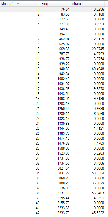
All the vibrations were inspected (they can found following this link), making sure that none of them were imaginary and the IR spectrum was simulated, as shown here below.

Energies under vibrational temperatures were recorded, as shown here below. The 'sum of electronic and zero-point energies' takes into account the zero-point vibrational energy (E0 = Eelec + ZPE), while the 'sum of electronic and thermal energies' includes the relative contributions of the translational, rotational, and vibrational modes(E = E0 + Evib + Erot + Etrans). The third and fourth values also contain additional correction terms: the 'sum of electronic and thermal enthalpies' accounts for thermal energy (H = E + RT)(which is particularly important when looking at dissociation reactions), whilst the 'sum of electronic and thermal free energies' includes the entropic contribution to the free energy (G = H - TS)[4]. All the energies are being thermally corrected, except the first one which is calculated at 0K.
Sum of electronic and zero-point Energies=           -234.469182
Sum of electronic and thermal Energies=              -234.461850
Sum of electronic and thermal Enthalpies=            -234.460906
Sum of electronic and thermal Free Energies=         -234.500698
These quantities were re-calculated at 0 K and by directly modifying the input file (which can be found following these links: 0K) and running the frequency analysis again. As shown here below, the first value remains constant as the temperature is varied as the 'Sum of electronic and zero-point Energies' is calculated at 0K. Also, at 0 K all the energy values are equal; this because, at absolute, there will be no additional contributions from the translational, rotational and vibrational modes. And similarly there will be no additional thermal energy that might contribute to the total energy of the system (H = E + RT, where T=0K so H=E!).
| 298.15 K | 0.000 K | |
|---|---|---|
| Link to Output File | log | log |
| Sum of electronic and zero-point Energies | -234.469182 | -234.469182 |
| Sum of electronic and thermal Energies | -234.461850 | -234.469182 |
| Sum of electronic and thermal Enthalpies | -234.460906 | -234.469182 |
| Sum of electronic and thermal Free Energies | -234.500698 | -234.469182 |
Conformers of 1,5-hexadiene
There are twelve rotational isomers of 1,5-hexadiene, among which two are enantiomeric pairs[3]. Therefore, all ten energetically different conformers were created with GaussiView and optimised the Hartree Fock method and the 3-21G basis set, in order to compare their relative energies. As expected, all conformers have relatively similar energies. Also, Gauche 3 has the lowest energy, and is the thus the most stable conformer. This is because of reduced steric clash between the vinyl protons and favourable π interaction between the terminal allylic[2], which could not occur in Anti 2, for example, in which both alkenes are pointing away from each other. Finally, Gauche 1, 5 & 6, and Anti 3 & 4 have higher energies than the other conformers because of greater unfavourable steric interactions between the vinyl protons. It is worth noting, that the relative energies differ from those found by B. W. Gung, Z. Zhu, and R. A. Fouch, but their ordering is identical [3]. This may due to the difference in methods that were use to run the calculations.
| Conformer | Structure | Links to Output Files | Point Group | Energy (a.u.) | Relative Energy (kcal/mol) |
|---|---|---|---|---|---|
| Gauche 1 |  |
log/ chk | C2 | -231.68771615 | 3.10 (3.10309) |
| Gauche 2 |  |
log/ chk | C2 | -231.69166689 | 0.62 (0.623994) |
| Gauche 3 |  |
log/ chk | C1 | -231.69266120 | 0.00 (0.000000) |
| Gauche 4 |  |
log /chk | C2 | -231.69153032 | 0.71 (0.709650) |
| Gauche 5 |  |
log/ chk | C1 | -231.68961573 | 1.91 (1.91108) |
| Gauche 6 |  |
log/ chk | C1 | -231.68916017 | 2.20 (2.19697) |
| Anti 1 |  |
log/ chk | C2 | -231.69260220 | 0.04 (0.037023) |
| Anti 2 |  |
log/ chk | Ci | -231.69253528 | 0.08 (0.079066) |
| Anti 3 |  |
log/ chk | C2h | -231.68907065 | 2.25 (2.225313) |
| Anti 4 |  |
log/ chk | C1 | -231.69097054 | 1.06 (1.06093) |
Optimisation of the chair and boat transition states
This section involved optimising the 'chair' and 'boat' transition state structures, in order to visualise the reaction coordinate, run the IRC (Intrinisic Reaction Coordinate) and calculate the activation energies for the Cope rearrangement.
Optimisation of an Allyl Fragment
| Molecule | 
|
| Links to output files | log/ chk |
| Calculation Type | FOPT |
| Calculation Method | UHF |
| Basis set | 3-21G |
| Final Energy (a.u.) | -115.82303994 |
| RMS Gradient Norm (a.u.) | 0.00008791 |
| Dipole Moment (Debye) | 0.0293 |
| Point Group | C1 |
| Point Group (after symmetrisation) | C2v |
| Time of calculation (s) | 24.0 |
An allyl fragment was created and then optimised using the Hartree Fock method and 3-21G basis set.
The RMS gradient was found to be close to zero (0.00008791 a.u.), meaning that the molecule had been successfully optimised. This was further confirmed by looking at the convergence of the forces and displacements in the output files, as shown here below.
        Item               Value     Threshold  Converged?
Maximum Force            0.000102     0.000450     YES
RMS     Force            0.000049     0.000300     YES
Maximum Displacement     0.000791     0.001800     YES
RMS     Displacement     0.000306     0.001200     YES
Predicted change in Energy=-1.644639D-07
Optimization completed.
   -- Stationary point found.
Optimisation of the Chair Transition State
Optimisation by Computing the Hessian
The 'chair' transition state was first optimised using a method known as the Hessian. This is the preferred method as it is the easiest, but it requires to guess the transition state's geometry reasonably well. Indeed, it computs the force constant matrix in the first step of the optimisation, and the guessed structure is then revised as the optimisation proceeds[4].
| Molecule | 
|
| Links to output files | log/ chk |
| Calculation Type | FOPT |
| Calculation Method | RHF |
| Basis set | 3-21G |
| Final Energy (a.u.) | -231.61932239 |
| RMS Gradient Norm (a.u.) | 0.00003300 |
| Dipole Moment (Debye) | 0.0005 |
| Point Group | C1 |
| Point Group (after symmetrisation) | C2h |
| Time of calculation (s) | 10.0 |
The previously optimised allyl fragment was duplicated and both fragments were oriented such that they would like the 'chair' transition state, making sure that the terminal ends of the allyl fragments were seperated by approximately 2.2 Å. The transition state was then optimised using the Hartree Fock method and 3-21G basis set. To do so, the 'Optimisation' command was set to a 'TS (Berny)', force constants were only calculated once, and the additional keywords Opt=NoEigen were included, to prevent the calculation from stopping if more than one imaginary frequency is detected.
The RMS gradient was found to be close to zero (0.00008791 a.u.), meaning that the molecule had been successfully optimised. This was further confirmed by looking at the convergence of the forces and displacements in the output files, as shown here below.
        Item               Value     Threshold  Converged?
Maximum Force            0.000065     0.000450     YES
RMS     Force            0.000015     0.000300     YES
Maximum Displacement     0.001493     0.001800     YES
RMS     Displacement     0.000342     0.001200     YES
Predicted change in Energy=-8.532989D-08
Optimization completed.
   -- Stationary point found.
As shown in the summary table, the obtained structure looked like a 'chair' transition state, and symmetrisation of the structure gave the C2h point group, as expected[5].
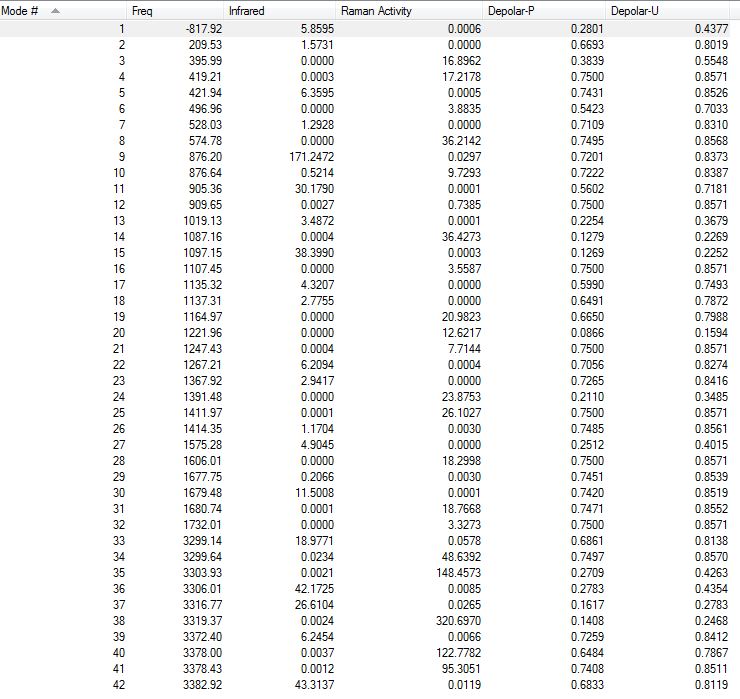
All the vibrations were inspected (they can be found following this link). As predicted and showed here below on an extract of the output file, the frequency calculation resulted in one imaginary frequency of magnitude -818 cm-1, meaning that job was successfully completed.
Low frequencies --- -817.9217   -2.6549   -0.0006    0.0004    0.0005    3.7756
Low frequencies ---    4.5940  209.5310  395.9867
This vibration, shown on the animation here below, correponds to the Cope rearrangement.

Optimisation by Freezing the Coordinates
The 'chair' structure was then optimised using a second method, as the first one often fails and/or leads to misleading results especially when the guess transition structure is far from the exact one. This time the transition structure was generated by freezing the reaction coordinate (using Opt=ModRedundant) and minimizing the rest of the molecule. After the molecule had fully relaxed, the reaction coordinate was unfrozened and the transition state was further optimised. Differentiating along the reaction coordinate was then sufficient to give a good guess for the initial force constant matrix, without having the need to compute the whole Hessian, and hence saving a considerable amount of time[4].
| Molecule | 
|
| Links to output files | log/ chk |
| Calculation Type | FOPT |
| Calculation Method | RHF |
| Basis set | 3-21G |
| Final Energy (a.u.) | -231.61465223 |
| RMS Gradient Norm (a.u.) | 0.00395651 |
| Dipole Moment (Debye) | 0.0044 |
| Point Group | C1 |
| Time of calculation (s) | 25.0 |
The guess structure of the 'chair' transition state was copied and pasted in GaussView. The terminal carbons from the allyl fragments which form/break a bond during the rearrangment were frozen. This was done by selecting 'Bond' instead of 'Unidentified' and 'Freeze Coordinate' instead of 'Add' in the Redundant Coordinate Editor. The transition structure was then optimised with the option Opt=ModRedundant.
The RMS gradient was found to be close to zero (0.00395651 a.u.), meaning that the molecule had been successfully optimised. This was further confirmed by looking at the convergence of the forces and displacements in the output files, as shown here below.
        Item               Value     Threshold  Converged?
Maximum Force            0.000060     0.000450     YES
RMS     Force            0.000014     0.000300     YES
Maximum Displacement     0.001306     0.001800     YES
RMS     Displacement     0.000383     0.001200     YES
Predicted change in Energy=-7.406912D-08
Optimization completed.
   -- Stationary point found.
As shown by GaussView's snapshot (in the summary table), the optimised structure was similar to the transition state previously optimised using Hessian's method, except that the bond forming/breaking distances were fixed to 2.2 Å.
| Molecule | 
|
| Links to output files | log/ chk |
| Calculation Type | FTS |
| Calculation Method | RHF |
| Basis set | 3-21G |
| Final Energy (a.u.) | -231.61932219 |
| RMS Gradient Norm (a.u.) | 0.00005611 |
| Dipole Moment (Debye) | 0.0006 |
| Point Group | C1 |
| Point Group (after symmetrisation) | C2h |
| Time of calculation (s) | 22.0 |
Bonds distances of the previous structure were optimised by selecting the frozen bonds and selecting 'Bond' instead of 'Unidentified' and 'Derivative' instead of 'Add', in the Redundant Coordinate Editor. A transition state optimisation was then carried out, but the force constants were not calculated as it was previously done. Instead, a modified normal guess Hessian was used, so that it would include information on the two coordinates along which we would be differentiating.
The RMS gradient was found to be close to zero (0.00005611 a.u.), meaning that the molecule had been successfully optimised. This was further confirmed by looking at the convergence of the forces and displacements in the output files, as shown here below.
        Item               Value     Threshold  Converged?
Maximum Force            0.000158     0.000450     YES
RMS     Force            0.000033     0.000300     YES
Maximum Displacement     0.001644     0.001800     YES
RMS     Displacement     0.000461     0.001200     YES
Predicted change in Energy=-2.404842D-07
Optimization completed.
   -- Stationary point found.
Comparison of the Chair Transition Structures
The chair transition structures obtained using different methods had relatively similar geometries: as shown in the table here below, the bond forming/bond breaking distances (C3-C4/C6-C1) only differed slightly. In fact, if those distances would even be equal if they were to be recorded with an 0.01 Å accuracy [1](2.02 Å). In the chair transition state, all bonds were equal to 1.39 Å; this was longer than the reactant's C=C double bonds (1.32 Å) but shorter than the the reactant's C-C single bonds (1.51 Å) due extended delocalisation throughout the allylic fragments. This was in agreement with the definition of a pericyclic of reaction, which should involved a cyclic transition state[6]. Moreover, the bonds distances that were calculated coïncide very well with the reported literature values, especially when using the Freezing Coordinates method (percentage errors of 0.9% for bond lengths and 3% for the bond breaking/ forming distance); this makes sense as this method is meant to be more accurate in finding a transition state structure. Finally the calculated bond breaking/ forming distance is very close to the experimental value of the actual transition state involved in the Cope rearrangement (percentage error of 2%); hence there is a high chance that the chair geometry is the real transition structure.
| Reactant (Anti 2) | Chair Transition State | ||||
|---|---|---|---|---|---|
| Hessian | Freezing Coordinates | Literature Values[5] | Experimental Values[5] | ||
| Structure |
|

| |||
| C1-C2/ C5-C6 | 1.32 (1.31613) | 1.39 (1.38931/ 1.38937) | 1.39 (1.38931) | 1.401 | |
| C2-C3/ C4-C5 | 1.51 (1.50891) | 1.39 (1.38920/ 1.38923) | 1.39 (1.38934) | 1.487 | |
| C3-C4/ C6-C1 (Bond Breaking/ Forming Distance) | 1.55/ NA (1.55275/ NA) | 2.02 (2.02069/ 2.02012) | 2.02 (2.01994/ 2.02065) | 2.086 | 2.062 |
Optimisation of the Boat Transition State
Using the QST2 Method
The 'boat' transition structure was then optimised, using the QST2 method. In this method, the reactants and products for a reaction need to be specified so that the calculation interpolates between the two structures to find the transition state located between them[4]. To do so, the optimised Ci anti 2 1,5-hexadiene reactant molecule, was duplicated, oriented and renumbered as shown here below, so that both the reactant and the product were numbered in the same way.
| Reactant | Product |
|---|---|
 |

|
A QST2 calculation was attempted, but the job failed: as shown by a snapshot of the checkpoint file, the obtained structure looked more like a dissociated chair transition structure (as illustrated by the relative bond distances: for example C1-C4 measures 2.02048 Å while it measures 2.01994 Å in the chair transition state) rather than a boat transition state.This is because this calculation resulted in a linear interpolation between the two structures: it simply translated the top allyl fragment without considering the possibility of a rotation around the central bonds[4].
 |
C1-C2/ C2-C3/ C4-C5/ C5-C6 |
1.39 (1.38928/ 1.38924/ 1.38930/ 1.38927) |
| C1-C4/ C3-C6 (Bond Forming/Breaking Distance) | 2.02 (2.02048/ 2.02054) |
Revisited QST2 Method
The reactant and product geometries were modified, so that they would look closer the 'boat' transition structure[4]. To do so, the central C-C-C-C dihedral angle was set to 0o and the inside C-C-C angle was set to 100o. This gave the following geometries for the reactant and product:
| Reactant | Product |
|---|---|
 |

|
| Molecule | 
|
| Links to output files | log/ chk |
| Calculation Type | FREQ |
| Calculation Method | RHF |
| Basis set | 3-21G |
| Final Energy (a.u.) | -231.60280170 |
| RMS Gradient Norm (a.u.) | 0.00008819 |
| Dipole Moment (Debye) | 0.1578 |
| Point Group | Cs |
| Point Group (after symmetrisation) | C2h |
| Time of calculation (s) | 6.0 |
A QST2 calculation was set up again, and, this time, the job successfully converged to the boat transition structure. The log file was examined to ensure that all the forces and displacements had converged:
The RMS gradient was found to be close to zero (0.00008819 a.u.), meaning that the molecule had been successfully optimised. This was further confirmed by looking at the convergence of the forces and displacements in the output files, as shown here below.
        Item               Value     Threshold  Converged?
Maximum Force            0.000093     0.000450     YES
RMS     Force            0.000034     0.000300     YES
Maximum Displacement     0.001171     0.001800     YES
RMS     Displacement     0.000374     0.001200     YES
Predicted change in Energy=-5.705714D-07
Optimization completed.
   -- Stationary point found.
As shown in the summary table, the obtained structure looked like a 'boat' transition state, and symmetrisation of the structure gave the C2v point group, as expected[5].
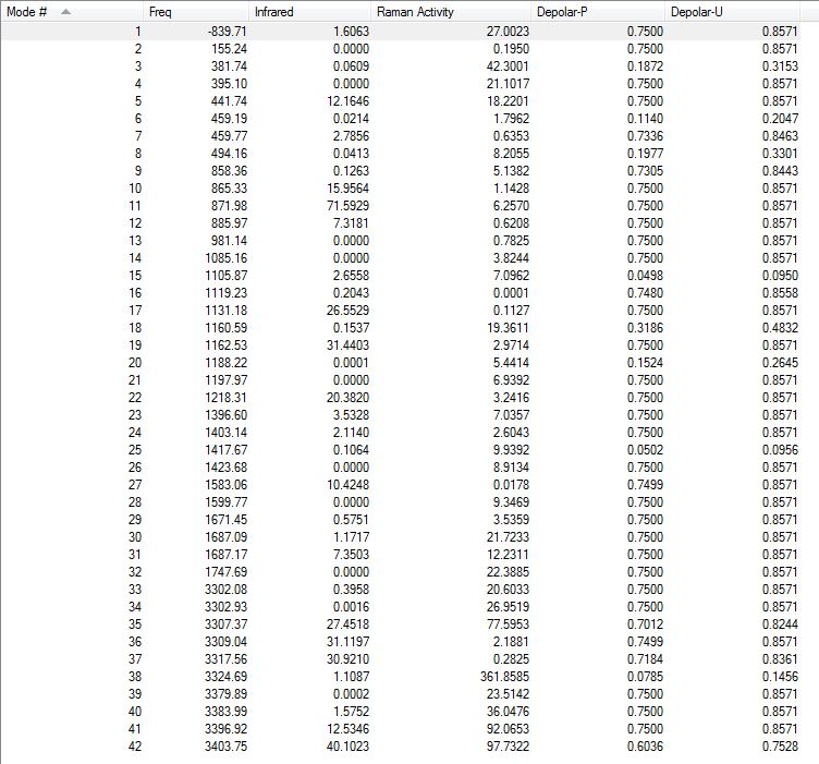
All the vibrations were inspected (they can be found following this link). As predicted and showed here below on an extract of the output file, the frequency calculation resulted in one imaginary frequency of magnitude-840 cm-1, meaning that job was successfully completed.
Low frequencies --- -839.7702   -5.7517   -0.0022   -0.0011   -0.0002    2.7352
Low frequencies ---    2.8938  155.2451  381.9359
An animation of the correspoding vibration is shown here below:

Using the QST3 Method
Although the QST2 method, has some advantages, for instance, it is fully automated, it can often fail if the reactants and/or products are not close to the transition structure[4]. As a result a more reliable method, called the QST3 method, which allows you to input the geometry of a guess transition structure[4], has been used for the next calculations. As previously, the guess transition structure was renumbered, as followed, so that its numbering would match the ones of the reactant and product.

| Molecule | 
|
| Links to output files | log/ chk |
| Calculation Type | FREQ |
| Calculation Method | RHF |
| Basis set | 3-21G |
| Final Energy (a.u.) | -231.60280240 |
| RMS Gradient Norm(a.u.) | 0.00001888 |
| Dipole Moment(Debye) | 0.1583 |
| Point Group | C1 |
| Point Group (after symmetrisation) | C2v |
| Time of calculation (s) | 9.0 |
The RMS gradient was found to be close to zero (0.00001888 a.u.), meaning that the molecule had been successfully optimised. This was further confirmed by looking at the convergence of the forces and displacements in the output files, as shown here below.
        Item               Value     Threshold  Converged?
Maximum Force            0.000036     0.000450     YES
RMS     Force            0.000010     0.000300     YES
Maximum Displacement     0.001264     0.001800     YES
RMS     Displacement     0.000381     0.001200     YES
Predicted change in Energy=-9.148480D-08
Optimization completed.
   -- Stationary point found.
All vibrations were inspected (they can be found following this link) and examination of the log file confirmed the presence of one imaginary frequency of magnitude -840 cm-1, as shown here below.
Low frequencies --- -839.7050   -4.0403   -0.0011   -0.0007   -0.0005    1.4918
Low frequencies ---    3.1183  155.2438  381.7431
Comparison of the Boat Transition Structures
The boat transition structures obtained using different methods had relatively similar geometries: as shown in the table here below, the bond forming/breaking distances (C3-C4/C6-C1) only differed slightly. In fact, if those distances would even be equal if they were to be recorded with an 0.01 Å accuracy[1] (2.14 Å). Similarly to the chair transition state, all bonds were equal to 1.38 Å; this was longer than the reactant's C=C double bonds (1.32 Å) but shorter than the the reactant's C-C single bonds (1.51 Å) due extented delocalisation throughout the allylic fragments; in agreement with the definition of a pericylic of reaction[6]. Moreover, the bonds distances that were calculated coïncide very well with reported literature values: percentage errors of 0.6% for the bond lengths and 7.6% for the bond breaking/ forming distance. The calculated bond breaking/ forming distance is still very close to the experimental value of the the actual transition state involved in the Cope rearrangement (percentage error of 3.8%); hence, the boat geometry could also be the real transition structure.
| Reactant (Anti 2) | Boat Transition State | ||||
|---|---|---|---|---|---|
| QST2 | QST3 | Literature Values[5] | Experimental Values[5] | ||
| Structure | |

| |||
| C1-C2/ C5-C6 | 1.32 (1.31613) | 1.38 (1.38140) | 1.38 (1.38143/ 1.38144) | 1.390 | |
| C2-C3/ C4-C5 | 1.51 (1.50891) | 1.38 (1.38128) | 1.38 (1.38136/ 1.38140) | 1.390 | |
| C3-C4/ C6-C1 (Bond Forming/ Breaking Distance) | 1.55/ NA (1.55275/ NA) | 2.14 (2.14118/ 2.14040) | 2.14 (2.14050/ 2.14042) | 2.316 | 2.062 |
Intrinsic Reaction Coordinates
The IRC or Intrinsic Reaction Coordinate method was then used to predict from which conformer of 1,5-hexadiene, the chair transition structure was originated. Indeed, the IRC can predict, from the transitions structures, which conformer the reaction paths will lead to. It follows the minimum energy path from a transition structure, by taking small geometry steps in the direction where the slope of the potential energy surface is steepest, until it reaches a local minimum [4].
| Molecule |  
|
| Links to output files | log/ chk |
| Calculation Type | IRC |
| Calculation Method | - |
| Basis set | 3-21G |
| Final Energy (a.u.) | -231.69157203 |
| RMS Gradient Norm (a.u.) | 0.00014489 |
| Dipole Moment (Debye) | 0.3622 |
| Point Group | C1 |
| Time of calculation | 5 min 25.0 s |
The IRC method was carried out on the optimised 'chair' transition structure. This was done by selecting 'IRC' under the Job Type tab, computing the reaction coordinate in the forward direction (as the reaction coordinate was symmetrical) and calculating the force constants at every step along the IRC. The IRC was first runned with a total number of 50 points. Calculations stopped at the last step (set 49). When running the IRC a second time, with a greater number of points (70), calculations also stopped at step 49, indicating at we had reached a local minimum on the potential energy surface.
A normal minimisation calculation was therefore runned on this point: the structure was first optimised using the Hartree Fock method with a 3-21G basis set and then further optimised using the B3LYP/6-31G(d) level of theory. This resulted in Gauche 2 conformer, as illustrated by the geometries and energies of the final structures. Comparison between both structures can be here found below: bond lengths and bond angles for both structures differed sligthly when using a HF/3-21G level of theory but turned out to be identical when using a B3LYP/6-31G(d)level of theory.

| ||
| Links to output files | log/ chk | log/ chk |
| Calculation Type | FOPT | FOPT |
| Calculation Method | RHF | RB3LYP |
| Basis set | 3-21G | 6-31G(d) |
| Final Energy (a.u.) | -231.69166702 | -234.61068493 |
| RMS Gradient Norm (a.u.) | 0.00000482 | 0.00003791 |
| Dipole Moment (Debye) | 0.3806 | 0.4392 |
| Point Group | C1 | C1 |
| Time of calculation (s) | 31.0 | 1 min 10.0 s |
Both RMS gradients were found to be close to zero (0.00000482 & 0.00003791 a.u.), meaning that structures were successfully optimised, which was further confirmed by looking at the convergence of the forces and displacements in the output files, as shown here below.
        Item               Value     Threshold  Converged?
Maximum Force            0.000010     0.000450     YES
RMS     Force            0.000003     0.000300     YES
Maximum Displacement     0.000291     0.001800     YES
RMS     Displacement     0.000087     0.001200     YES
Predicted change in Energy=-2.429908D-09
Optimization completed.
   -- Stationary point found.
        Item               Value     Threshold  Converged?
Maximum Force            0.000069     0.000450     YES
RMS     Force            0.000021     0.000300     YES
Maximum Displacement     0.001723     0.001800     YES
RMS     Displacement     0.000512     0.001200     YES
Predicted change in Energy=-7.387487D-08
Optimization completed.
   -- Stationary point found.
| IRC Result | Gauche 2 | |||
|---|---|---|---|---|
| HF/ 3-21G | B3LYP/ 6-31G(d) | HF/ 3-21G | B3LYP/ 6-31G(d) | |
| Structure | 
| |||
| Energies | -231.69166689 | -234.61068493 | -231.69166702 | -234.61068493 |
| C1-C2/ C5-C6 | 1.32 (1.31566) | 1.33 (1.33302) | 1.31 (1.31562/ 1.31542) | 1.33 (1.33302) |
| C3-C4 | 1.55 (1.55082) | 1.55 (1.54833) | 1.55 (1.55086) | 1.55 (1.54833) |
| C2-C3/ C4-C5 | 1.51 (1.50829) | 1.51 (1.50816) | 1.51 (1.50823/ 1.50837) | 1.50 (1.50438) |
| C1-C2-C3/ C4-C5-C6 | 125.0 (124.975) | 125.4 (125.416) | 125.0 (124.978/ 124.981) | 125.4 (125.416) |
| C2-C3-C4/ C3-C4-C5 | 112.0 (112.041) | 113.6 (113.635) | 112.0 (112.034/ 112.037) | 113.6 (113.635) |
Activation Energies
Optimisation of the Chair and Boat Transition States using a higher level of theory
To calculate the activation energies for the reaction via the chair and boat transition structures, both transition structures were reoptimised using the B3LYP/6-31G(d) level of theory.
| Chair | Boat | |
|---|---|---|
| Molecule |  |

|
| Link to output file | log | log |
| Calculation Type | FREQ | |
| Calculation Method | RB3LYP | |
| Basis set | 6-31G(d) | |
| Final Energy (a.u.) | -234.55698303 | -234.54309307 |
| RMS Gradient Norm (a.u.) | 0.00001194 | 0.00000444 |
| Dipole Moment (Debye) | 0.4392 | 0.0613 |
| Point Group | C1 | C1 |
| Point Group (after symmetrisation) | C2h | C2v |
| Time of calculation | 5 min 43.8 s | 5 min 36.5 s |
Both RMS gradients were found to be close to zero (0.00001194 & 0.00000444 a.u.), meaning that structures were successfully optimised, which was further confirmed by looking at the convergence of the forces and displacements in the output files, as shown here below.
        Item               Value     Threshold  Converged?
Maximum Force            0.000023     0.000450     YES
RMS     Force            0.000005     0.000300     YES
Maximum Displacement     0.000075     0.001800     YES
RMS     Displacement     0.000025     0.001200     YES
Predicted change in Energy=-3.724413D-09
Optimization completed.
   -- Stationary point found.
        Item               Value     Threshold  Converged?
Maximum Force            0.000009     0.000450     YES
RMS     Force            0.000003     0.000300     YES
Maximum Displacement     0.000169     0.001800     YES
RMS     Displacement     0.000054     0.001200     YES
Predicted change in Energy=-3.423638D-09
Optimization completed.
   -- Stationary point found.
Comparison of the Chair and Boat Structures
As shown in the table here below, calculated bond lengths coïncide perfectly with reported literature values, especially when using the [B3LYP/6-31G(d)] high level of theory. Looking at the bond forming/ breaking distance of the chair and boat transition states and comparing them to experimental value of 2.086 Å [HF/3-21G] suggests that the Cope rearrangement occurs through a concerted fashion via a 'chair' transition state.
| Chair TS | Boat TS | |||
|---|---|---|---|---|
| Structures | |
| ||
| HF/3-21G | B3LYP/6-31G(d) | HF/3-21G | B3LYP/6-31G(d) | |
| C1-C2/ C2-C3/ C4-C5/ C5-C6 | 1.39 [lit. 1.401][5] | 1.41 | 1.38 [lit. 1.390][5] | 1.39 |
| C3-C4/ C6-C1 (Bond Forming/Breaking Distance) | 2.02 [lit. 2.086][5] | 1.97 [lit. 1.971][7] | 2.14 [lit. 2.316][5] | 2.21 [lit. 2.208][7] |
Calculation of the Activation Energies
Summary of energies (a.u.)
| HF/3-21G | B3LYP/6-31G* | |||||
|---|---|---|---|---|---|---|
| Electronic energy | Sum of electronic and zero-point energies | Sum of electronic and thermal energies | Electronic energy | Sum of electronic and zero-point energies | Sum of electronic and thermal energies | |
| at 0 K | at 298.15 K | at 0 K | at 298.15 K | |||
| Chair TS | -231.619322 | -231.466701 | -231.461342 | -234.556983 | -234.414929 | -234.409009 |
| Boat TS | -231.602802 | -231.450930 | -231.445300 | -234.543093 | -234.402342 | -234.396008 |
| Reactant (anti2) | -231.692535 | -231.539539 | -231.532565 | -234.611712 | -234.469182 | -234.461850 |
Summary of activation energies (kcal/mol)
| HF/3-21G | HF/3-21G | B3LYP/6-31G* | B3LYP/6-31G* | Expt.[8] | |
| at 0 K | at 298.15 K | at 0 K | at 298.15 K | at 0 K | |
| ΔE (Chair) | 45.71 | 44.69 | 34.04 | 33.16 | 33.5 ± 0.5 |
| ΔE (Boat) | 55.60 | 54.76 | 41.94 | 41.32 | 44.7 ± 2.0 |
The activation energies at 0 K were calculated by subtracting the 'sum of electronic and zero-point energies' of the reactant/ Anti 2 to 'sum of electronic and zero-point energies' of the transition states.The obtained values fit very well with the experimental ones, especially when using a B3LYP/6-31G(d) level of theory. Because 6-31G(d) is a higher basis set it gives more accurate results: using a HF/3-21G level of theory leads to percentage errors of respectively 36.4% and 24.4% for the chair and boat transition states, whilst using using a B3LYP/6-31G(d) level of theory leads to percentage errors of respectively 1% and 6.2% for the chair and boat transition states.
The chair transition state is 10.37 kcal/mol [HF/3-21G] /8.710 kcal/mol [B3LYP/6-31G(d)] lower in energy than the boat one (this is larger than the expected value of 5.8 kcal/mol[9] but it can be due to the difference in basis sets). This suggests that the chair geometry is the preferred one and hence supports the 'classical rules'[7] of Cope rearrangement. Usually, the stability of the chair conformer relative to the boat one would be explained giving two reasons: the first one being that in the boat conformation the horizontal CC bonds are eclipsed, whilst in the chair conformation, all the bonds are staggered, leading to a higher degree of torsional strain in the boat conformation[10]. The second reason would involve the close proximity of the 'flagpole or bowsprit' hydrogens[11] (only 1.80 Å[10] apart from each other) by and hence additional Van der Waals repulsion, as illustrated here below.

However, in the obtained boat transition structure, both hydrogens are seperated by 3.23 Å, which is larger than 2.40 Å, i.e. twice hydrogen's Van der Waals radius [12]. Therefore, the previous explanation appears unsatisfactory and the another electronic effect should be considered in order to explain the preference of the chair geometry relative to the boat one in the Cope rearrangement.
According to Woodward and Hofmann's symmetry rules, the Cope rearrangement is a thermally allowed pericyclic reaction, which should pass through an aromatic transition state [6]. Doering and Roth showed that, even though, the boat transition state involved a '6-atom-arrangement' of the two parallel allylic groups, it was higher in energy than chair transition state, which involved a '4-atom-arrangement' in which both ends only of the allylic system interact [13]. In fact, this can be explained by looking at the frontier orbitals and more specifically at the ‘secondary interactions’ [14] in the Cope rearrangement. As shown here below, in the boat transition state there is an extra antibonding interaction between the C2 and C5's lobes [14]; this unfavourable interaction raises the energy of the system relative to the chair transition state, in which these lobes are too far apart to interact. Therefore, the chair geometry is lower in energy, its activation barrier is smaller, and hence, the rate constant of its formation is larger (from Arrhenius equation [15]). This explains why the chair transition state is preferred over the boat one in the Cope rearrangement.

THE DIELS-ALDER CYCLOADDITION
The second part of this project involved an in-depth study of another pericyclic reaction known as the Diels-Alder reaction, which is a [π4s +π2s] cycloaddition. Its reactivity and stereospecificity was explored by characterising the transition structures and examining the molecular orbitals of two different examples.
Diels-Alder Reaction between Cis-Butadiene and Etylene
The reaction of Cis-Butadiene with Ethylene, illustrated here below, was first considered.

Optimisation of the Reactants
Optimisation Cis-Butadiene
A molecule of cis-butadiene was created in Gaussview and optimised using the semi-empirical AM1 molecular orbtital method. It was then reoptimised using higher levels of theory: HF/3-21G followed B3LYP/6-31G(d). All RMS gradients were found to be close to zero (0.0011857, 0.0011857 & 0.00003238 a.u.), meaning that structures were successfully optimised, which was further confirmed by looking at the convergence of the forces and displacements in the output files, as shown here below.
| 1st Optimisation | 2nd Optimisation | 3rd Optimisation | |
|---|---|---|---|
| Molecule |  | ||
| Links to output files | log/ chk | log/ chk | log/ chk |
| Calculation Type | FOPT | FOPT | FOPT |
| Calculation Method | RAM1 | RHF | RB3LYP |
| Basis set | ZDO | 3-21G | 6-31G(d) |
| Final Energy (a.u.) | 0.04879734 | -154.05394305 | -155.98594961 |
| RMS Gradient Norm (a.u.) | 0.00008900 | 0.0011857 | 0.00003238 |
| Dipole Moment (Debye) | 0.0414 | 0.0338 | 0.0852 |
| Point Group | C1 | ||
| Point Group (after symmetrisation) | C2v | ||
| Time of calculation (s) | 35.0 | 23.0 | 40.0 |
        Item               Value     Threshold  Converged?
Maximum Force            0.000159     0.000450     YES
RMS     Force            0.000051     0.000300     YES
Maximum Displacement     0.000661     0.001800     YES
RMS     Displacement     0.000254     0.001200     YES
Predicted change in Energy=-1.540760D-07
Optimization completed.
   -- Stationary point found.
        Item               Value     Threshold  Converged?
Maximum Force            0.000239     0.000450     YES
RMS     Force            0.000078     0.000300     YES
Maximum Displacement     0.000995     0.001800     YES
RMS     Displacement     0.000343     0.001200     YES
Predicted change in Energy=-2.308366D-07
Optimization completed.
   -- Stationary point found.
        Item               Value     Threshold  Converged?
Maximum Force            0.000073     0.000450     YES
RMS     Force            0.000023     0.000300     YES
Maximum Displacement     0.000266     0.001800     YES
RMS     Displacement     0.000132     0.001200     YES
Predicted change in Energy=-2.716651D-08
Optimization completed.
   -- Stationary point found.
Optimisation of Ethylene
| Molecule | 
|
| Links to output files | log/ chk |
| Calculation Type | FOPT |
| Calculation Method | RB3LYP |
| Basis set | 6-31G(d) |
| Final Energy (a.u.) | -78.58745746 |
| RMS Gradient Norm (a.u.) | 0.00014422 |
| Dipole Moment (Debye) | 0.0000 |
| Point Group | C1 |
| Point Group (after symmetrisation) | D2h |
| Time of calculation | 7.0 s |
A molecule of ethlyne was created in Gaussview and optimised using a B3LYP method and a 6-31G(d) basis set. Its RMS gradient was found to be close to zero (0.00014422 a.u.), meaning that the structure had been successfully optimised. This was further confirmed by looking at the convergence of the forces and displacements in the output files, as shown here below.
        Item               Value     Threshold  Converged?
Maximum Force            0.000230     0.000450     YES
RMS     Force            0.000136     0.000300     YES
Maximum Displacement     0.001375     0.001800     YES
RMS     Displacement     0.001006     0.001200     YES
Predicted change in Energy=-8.331632D-07
Optimization completed.
   -- Stationary point found.
Optimisation of the Product: Cyclohexene
| Molecule | 
|
| Links to output files | log/ chk |
| Calculation Type | FOPT |
| Calculation Method | RB3LYP |
| Basis set | 6-31G(d) |
| Final Energy (a.u.) | -234.63289313 |
| RMS Gradient Norm (a.u.) | 0.00007877 |
| Dipole Moment (Debye) | 0.3498 |
| Point Group | C1 |
| Point Group (after symmetrisation) | C2v |
| Time of calculation | 1 min 31.0 s |
A molecule of cyclohexene was created in GaussView and optimised using a B3LYP method and 6-31G(d)basis set. The RMS gradient was found to be close to zero (0.00007877 a.u.), meaning that the structure had been successfully optimised. This was further confirmed by looking at the convergence of the forces and displacements in the output files, as shown here below.
        Item               Value     Threshold  Converged?
Maximum Force            0.000207     0.000450     YES
RMS     Force            0.000044     0.000300     YES
Maximum Displacement     0.000975     0.001800     YES
RMS     Displacement     0.000252     0.001200     YES
Predicted change in Energy=-2.989012D-07
Optimization completed.
   -- Stationary point found.
Optimisation of the Transition State
The transition state was optmised using two different methods.
Using the Hessian Method
The previously optimised cis-butadiene and ethylene fragments were oriented such that they would like the required transition state, seperating terminal ends by approximately 2.2 Å. The transition state was then optimised using the Hartree Fock method and 3-21G basis set. To do so, the 'Optimisation' command was set to a TS (Berny)', force constants were only calculated once, and the additional keywords Opt=NoEigen were included. The obtained structure was then further optimised using a higher level of theory: B3LYP/6-31G(d).
| 1st Optimisation | 2nd Optimisation | |
|---|---|---|
| Molecule |  
| |
| Links to output files | log | log/ chk |
| Calculation Type | FREQ | FREQ |
| Calculation Method | RHF | RB3LYP |
| Basis set | 3-21G | 6-31G(d) |
| Final Energy (a.u.) | -231.60320857 | -234.54389653 |
| RMS Gradient Norm (a.u.) | 0.00000342 | 0.00001338 |
| Dipole Moment (Debye) | 0.5757 | 0.3943 |
| Point Group | C1 | |
| Point Group (after symmetrisation) | Cs | |
| Time of calculation (s) | 21.6 | 40.0 |
Both RMS gradients were found to be close to zero (0.00000342 & 0.00001338 a.u.), meaning that structures were successfully optimised, which was further confirmed by looking at the convergence of the forces and displacements in the output files, as shown here below.
        Item               Value     Threshold  Converged?
Maximum Force            0.000014     0.000450     YES
RMS     Force            0.000002     0.000300     YES
Maximum Displacement     0.000030     0.001800     YES
RMS     Displacement     0.000009     0.001200     YES
Predicted change in Energy=-3.866693D-10
Optimization completed.
   -- Stationary point found.
        Item               Value     Threshold  Converged?
Maximum Force            0.000030     0.000450     YES
RMS     Force            0.000006     0.000300     YES
Maximum Displacement     0.000625     0.001800     YES
RMS     Displacement     0.000172     0.001200     YES
Predicted change in Energy=-2.365409D-08
Optimization completed.
   -- Stationary point found.
Using the QST3 Method
The guessed transition structure was then optimised using the QST3 method with the B3LYP/6-31G(d)level of theory. To do so, both reactants and the product were used in the input file.
| Molecule |  
|
| Links to output files | log/ chk |
| Calculation Type | FREQ |
| Calculation Method | RB3LYP |
| Basis set | 6-31G(d) |
| Final Energy (a.u.) | -234.54389655 |
| RMS Gradient Norm (a.u.) | 0.00001904 |
| Dipole Moment (Debye) | 0.3943 |
| Point Group | C1 |
| Point Group (after symmetrisation) | Cs |
| Time of calculation | 1 min 22.0 s |
The RMS gradient was found to be close to zero (0.00001904 a.u.), meaning that the structure had been successfully optimised, which was further confirmed by looking at the convergence of the forces and displacements in the output files, as shown here below.
        Item               Value     Threshold  Converged?
Maximum Force            0.000016     0.000450     YES
RMS     Force            0.000006     0.000300     YES
Maximum Displacement     0.001238     0.001800     YES
RMS     Displacement     0.000245     0.001200     YES
Predicted change in Energy=-8.219250D-09
Optimization completed.
   -- Stationary point found.
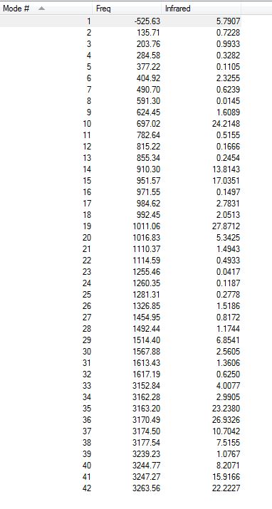
All the vibrations were inspected (they can be found following this link). As expected for a transition structure, the frequency calculation resulted in one imaginary frequency, of magnitude -526 cm-1, as shown here below, meaning that job was successfully completed.
Low frequencies --- -525.6297   -6.7129    0.0005    0.0006    0.0010   10.1114
Low frequencies ---   19.8223  135.7697  203.7765
This vibration corresponds to the Diels-Alder reaction. As shown here below, the bond forming/breaking occur synchronously in a concerted fashion. In this stretching mode, cis-butadiene and ethylene vibrate simultaneously as one entity, as if the molecule was already formed. This contrasts with the lowest positive frequency, occurring at 136 cm-1, in which both fragments clearly show separate motions. This twisting mode is a 'reaction pathway to the transition state'[4].
| Imaginary Frequency [-526 cm-1] | Lowest Positive Frequency [136 cm-1] |
|---|---|
 |

|
Comparison of the Different Transition State Structures
Bond forming/breaking distances of the optimised structures of the guessed transition state were tabulated. As shown here below, those distances are relatively similar using both methods of optimisation.
| Structure | Bonds | Reactants | Transition State (Hessian Method) | Transition State (QST3 Method) |
|---|---|---|---|---|
 |
C1-C2/C6-C7 |
1.34 (1.33985) [lit. 1.348][16] | 1.38 (1.38303/1.38306) | 1.38 (1.38310) |
C1-C6 |
1.47 (1.47144) [lit. 1.468][16] | 1.41 (1.40717) | 1.41 (1.40712) | |
C11-C12 |
1.33 (1.33071) [lit. 1.330][16] | 1.39 (1.38598) | 1.39 (1.38605) | |
C2-C11/C7-C12 |
- | 2.27 (2.27244/2.27234) | 2.27 (2.27175/2.27171) |
In the transition state, C2-C11 and C7-C12 bonds were are 2.27 Å long. This is longer than typical σ C-C bonds (1.530 Å[17]), but shorter than 3.4 Å, i.e. twice Van der Waals radii[12]; this suggested a favourable overlap of carbons' Van der Waals radii, leading to the formation of two new σ bonds. The fact that C2-C11 and C7-C12 bond lengths were identical confirmed that this process was happening in a concerted fashion. Ethylene's C=C double bond length was increased by 0.06 Å (C11-C12: 1.33->1.39 Å), whilst cis-butadiene's C=C double bond length was increased by 0.04 Å (C1-C2/C6-C7: 1.34->1.38 Å). This illustrated the breaking of the C=C double bonds and the formation of C-C single bond, which would occur through donation of ethylene π electron density into cis butadiene π*. On the contrary, C1-C6 bond length significantly dropped (1.47->1.41 Å) allowing carbon p orbitals' reorientation and hence better overlap. As a result, all allylic CC bond lengths were relatively similar [they were shorter than typical C-C bonds (1.530 Å[17]) but longer than C=C bonds (1.316 Å[17])], illustrating a high extent of delocalisation and hence confirming that the reaction was taking place via a cyclic transition state[6]. Finally, it is worth noting that the calculated bond lengths were very close to the experimental ones reported in the literature showing the high level of accuracy of the chosen method and basis set.
Frontier Orbitals
The HOMO and LUMO of both reactants and the transition state were visualised using the checkpoint file, in order to study the stereospecificity of Diels-Alder reaction.
| Cis-Butadiene | Ethylene | Transition State | |
|---|---|---|---|
| HOMO |  E= -0.22736 ANTISYMMETRIC |
 E= -0.26667 SYMMETRIC |
 SYMMETRIC |
| LUMO |  E= +0.01881 SYMMETRIC |
 E= -0.03013 ANTISYMMETRIC |
 SYMMETRIC |
| Cis-Butadiene | HOMO | LUMO |
| Ethylene | LUMO | HOMO |
| ΔE (HOMO-LUMO) | 0.24617 | 0.23654 |
The reaction of cis-butadiene with ethylene involves 4 π electrons from the former component and 2 from the latter ; it is a [4+2] cycloaddition [14] and hence belongs to a class of reactions known as the 'pericyclic reactions' [4]. Whether the reaction occurs in a concerted stereospecific fashion, and hence is allowed, depends on the relative symmetries of the Frontier Orbitals of both fragments. The HOMO-LUMO can only interact when there is a significant overlap density; therefore, if the orbitals have different symmetry properties, no overlap is possible, and hence the reaction is forbidden [14].
As shown by the different GaussiView snapshots, the HOMO of cis-butadiene and the LUMO of ethylene butadiene are both antisymmetric, while the LUMO of cis-butadiene and the HOMO of ethylene are both symmetric, with respect to a reflection plane bisecting the two central carbon of cis-butadiene. In theory, both sets of MOs could thus overlap and drive the reaction, as illustrated in the MO diagram here below. However, the HOMO of the transition state is symmetric with respect to the plane of symmetry; therefore, the combined orbitals must also be symmetric [4]. Hence, HOMO of the transition state results from the interaction of cis-butadiene’s LUMO with ethylene’s HOMO.
Usually, the diene is electron rich, and hence has a high-energy HOMO, while the dienophile, is electron poor, and hence has a low-energy LUMO, as this combination gives a better overlap in the transition state[18]. However, in this case, both, the diene and the dienophile, cis-butadiene and ethylene, respectively, are electron rich. Therefore, both HOMOs and both LUMOs are close in energy. As a result, there will not be much energy gain in interacting cis-butadiene’s HOMO with ethylene’s LUMO (versus cis-butadiene’s LUMO with ethylene’s HOMO). Energies of the relative Frontier Orbitals were inspected, and it turns out that, in fact, the energy difference [LUMO(cis-butadiene)-HOMO(ethylene)] is slightly smaller than [HOMO(cis-butadiene)-LUMO(ethylene)] (0.23654 a.u. compared to 0.24617 a.u.) (as illustrated by the table above).

A Study of the Regioselectivity of Diels-Alder Reaction between Cyclohexa-1,3-diene and Maleic Anhydride
The regioselectivity of Diels Alder's reaction was then investigated by looking at the reaction of Cyclohexa-1,3-diene with Maleic Anhydride. This reaction should lead to the formation of two products; however, under kinetic control, it should primarily give the endo adduct[4].

Optimisation of the Reactants and Products
Both reactants and products were optimised using a B3LYP method and a 6-31G(d) basis set.
| Cyclohexa-1,3-diene | Maleic Anhydride | Exo Adduct | Endo Adduct | |
|---|---|---|---|---|
| Molecule |  |
 |
 |

|
| Links to output files | log/ chk | log/ chk | log/ chk | log/ chk |
| FOPT | ||||
| RB3LYP | ||||
| 6-31G(d) | ||||
| Final Energy (a.u.) | -233.41588484 | -379.28954441 | -612.75578548 | -612.75829019 |
| RMS Gradient Norm (a.u.) | 0.00007566 | 0.00010583 | 0.00000675 | 0.00001632 |
| Dipole Moment (Debye) | 0.5484 | 4.0718 | 4.7598 | 5.0201 |
| Point Group | C1 | |||
| Point Group (after symmetrisation) | C2v | C2v | Cs | Cs |
| Time of calculation | 1 min 16.0 | 1 min 3.0 | 21 min 42.0 | 25 min 43.0 |
RMS gradients were found to be close to zero (0.00007566, 0.00010583, 0.00000675 & 0.00001632 a.u.), meaning that the structures were successfully optimised. This was further confirmed by looking at the convergence of the forces and displacements in the output files, as shown here below.
        Item               Value     Threshold  Converged?
Maximum Force            0.000275     0.000450     YES
RMS     Force            0.000038     0.000300     YES
Maximum Displacement     0.000532     0.001800     YES
RMS     Displacement     0.000141     0.001200     YES
Predicted change in Energy=-1.439580D-07
Optimization completed.
   -- Stationary point found.
        Item               Value     Threshold  Converged?
Maximum Force            0.000216     0.000450     YES
RMS     Force            0.000071     0.000300     YES
Maximum Displacement     0.000692     0.001800     YES
RMS     Displacement     0.000250     0.001200     YES
Predicted change in Energy=-2.569410D-07
Optimization completed.
   -- Stationary point found.
        Item               Value     Threshold  Converged?
Maximum Force            0.000019     0.000450     YES
RMS     Force            0.000004     0.000300     YES
Maximum Displacement     0.000814     0.001800     YES
RMS     Displacement     0.000143     0.001200     YES
Predicted change in Energy=-1.243639D-08
Optimization completed.
   -- Stationary point found.
        Item               Value     Threshold  Converged?
Maximum Force            0.000040     0.000450     YES
RMS     Force            0.000007     0.000300     YES
Maximum Displacement     0.001553     0.001800     YES
RMS     Displacement     0.000230     0.001200     YES
Predicted change in Energy=-2.658569D-08
Optimization completed.
   -- Stationary point found.
Optimisation of the Transition States
Structures of both transition states - the one corresponding to the exo adduct and the one corresponding to the endo adduct - were guessed and then optimised using the QST3 method. To do so, structures of the reactants, transition states and products, were added to the input files, renumbered and oriented properly. The Job title was changed to 'Opt+Freq', the 'Optimisation' command was set to a 'QTS3' and force constants were only calculated at every step (to maximise changes of finding of the transition state). The transition states were optimised using a B3LYP method and a 6-31G(d) basis set.
Optimisation of the Exo Transition State
| Molecule | 
|
| Links to output files | log/ chk |
| Calculation Type | FREQ |
| Calculation Method | RB3LYP |
| Basis set | 6-31G(d) |
| Final Energy (a.u.) | -612.67931096 |
| RMS Gradient Norm (a.u.) | 0.00000288 |
| Dipole Moment (Debye) | 5.5501 |
| Point Group | C1 |
| Point Group (after symmetrisation) | Cs |
| Time of calculation | 26 min 23.6 s |
The RMS gradient was found to be close to zero (0.00000288 a.u.), meaning that the structure was successfully optimised. This was further confirmed by looking at the convergence of the forces and displacements in the output files, as shown here below.
        Item               Value     Threshold  Converged?
Maximum Force            0.000004     0.000450     YES
RMS     Force            0.000001     0.000300     YES
Maximum Displacement     0.000434     0.001800     YES
RMS     Displacement     0.000126     0.001200     YES
Predicted change in Energy=-3.909007D-09
Optimization completed.
   -- Stationary point found.
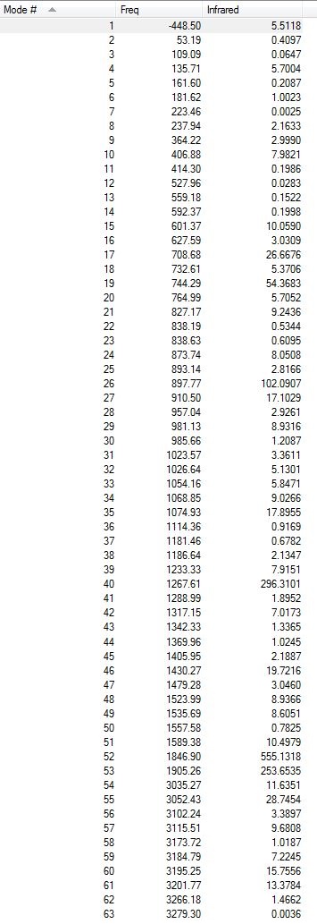
All the vibrations were inspected (they can be found following this link). As expected for a transition structure, the frequency calculation resulted in one imaginary frequency, of magnitude -448 cm-1, as shown here below, meaning that job was successfully completed.
Low frequencies --- -448.4969  -13.9288  -11.7631    0.0008    0.0009    0.0010
Low frequencies ---    3.0620   53.3059  109.0927
The animation of the corresponding vibration showed a synchronous reaction pathway[4], which is consistant with Woodward and Hofmann's symmetry rules[6].

Optimisation of the Endo Transition State
| Molecule | 
|
| Links to output files | log/ chk |
| Calculation Type | FOPT |
| Calculation Method | RB3LYP |
| Basis set | 6-31G(d) |
| Final Energy (a.u.) | -612.68339677 |
| RMS Gradient Norm (a.u.) | 0.00007877 |
| Dipole Moment (Debye) | 0.3498 |
| Point Group | C1 |
| Point Group | Cs |
| Time of calculation | 26 min 6.7 s |
The RMS gradient was found to be close to zero (0.00007877 a.u.), meaning that the structure was successfully optimised. This was further confirmed by looking at the convergence of the forces and displacements in the output files, as shown here below.
        Item               Value     Threshold  Converged?
Maximum Force            0.000003     0.000450     YES
RMS     Force            0.000000     0.000300     YES
Maximum Displacement     0.000359     0.001800     YES
RMS     Displacement     0.000066     0.001200     YES
Predicted change in Energy=-9.966983D-10
Optimization completed.
   -- Stationary point found.
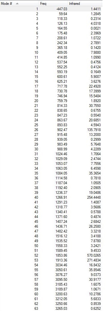
All the vibrations were inspected (they can be found following this link). As expected for a transition structure, the frequency calculation resulted in one imaginary frequency, of magnitude -447 cm-1, as shown here below, meaning that job was successfully completed.
Low frequencies --- -447.0280  -14.2619   -0.0004    0.0005    0.0005    4.5194
Low frequencies ---   11.2870   59.6502  118.3544
As for previously, the animation of the corresponding vibration showed a synchronous reaction pathway[4], which is consistant with Woodward and Hofmann's symmetry rules[6].

Comparison of the two Transition States
Bond Lengths
| Exo Transition State | Endo Transition State | |
|---|---|---|
| Structure |  |

|
| C1-C4 (Double Bond Forming) | 1.40 (1.40345) | 1.40 (1.40307) |
| C1-C2/C4-C3 (Double Bonds Breaking) | 1.39 (1.39140 / 1.39142) | 1.39 (1.39124 / 1.39125) |
| C2-C12/C3-C9 | 1.51 (1.51453) | 1.51 (1.51508) |
| C12-C9 | 1.56 (1.55839) | 1.56 (1.55823) |
| C3-C17/C2-C16 (Bond between cyclohexa-1,3-diene and maleic anhydride forming) | 2.29 (2.29046 / 2.29068) | 2.27 (2.26841/ 2.26829) |
| C16-C17 (Double Bond breaking) | 1.40 (1.39790) | 1.39 (1.39397) |
| Through space interaction | C9-C18/ C12-C15 3.02 (3.02793 / 3.02788) |
C1-C18/ C4-C15 2.99 (2.99007 / 2.99016) |
As shown in the table above, most of C-C bonds are of equal length, confirming that the reaction is taking place via a cyclic transition state[6]. C1-C4 bonds are shorter than single bonds (typical C-C 1.530 Å[17]), whilst C2-C12/ C3-9/ C16-C17/are longer than double bonds (typical C=C 1.316 Å[17]), indicating that the former are becoming double bonds, whilst the latter are breaking into single bonds in a concerted fashion. C3-C17 and C2-C16 are 2.29 and 2.27 Å long, for the exo and endo transition states respectively. Again, this is longer than typical C-C bonds but shorter than twice Van der Waals radii [12], indicating some sort of interaction, and suggesting the future presence of two σ bonds. It is worth noting that this calculated bond length is very close to the value reported in the literature for the endo transition state [2.265 Å][19] ; the small difference of 0.003 Å may simply arise from the difference in basis sets: 6-31G(d,p) compared to 6-31G(d).
The key difference between both transition states concerns the through space interaction: the C-C through space distance between the -(C=O)-O-(C=O)- fragment of the maleic anhydride and the C atoms of the 'opposite' -CH2-CH2- for the exo transition state is 3.03 Å, while the C-C through space distances between the -(C=O)-O-(C=O)- fragment of the maleic anhydride and the C atoms of the 'opposite' -CH=CH- for the endo transition state is 2.99 Å. This is because: in the exo transition state, the C=O bonds of maleic anhydride are pointing towards the π-system of the diene and thus away from the larger, and hence more hindered, bridge, while in the endo transition state the C=O bonds of maleic anhydride are pointing away the π-system of the diene and thus towards the larger bridge. This positioning also results in the close proximity of H10 and 13 to maleic anhydride’s ring : distanced by 2.53 Å (2.52974 and 2.52933 Å). As a result, the exo transition state is less sterically hindered and thermodynamically favoured[18].
Frontier Orbitals
To understand the regioselectivity of the Diels-Alder reaction, Frontier Orbitals of both reactants an both transition states were visualised using the checkpoint file.
| HOMO of Cyclohexa-1,3-diene | LUMO of Maleic Anhydride | |||
|---|---|---|---|---|
| MOs |  |
 |
 |

|
| Energies [B3LYP/6-31G(d)] | -0.20102 | -0.11709 | ||
| ΔE(HOMO-LUMO) | 0.31811 | |||
| Exo Transition State | Endo Transition State | |||
|---|---|---|---|---|
| HOMO |  ANTISYMMETRIC |
 E= -0.24216 |
 ANTISYMMETRIC |
 E= -0.24229 |
| LUMO |  ANTISYMMETRIC |
 E= -0.07840 |
 ANTISYMMETRIC |
 E= -0.0673 |
The reaction of cyclohexa-1,3-diene with maleic anhydride corresponds to a 'normal electron demand'[18]: cyclohexa-1,3-diene, the diene, is electron rich, while maleic anhydride, the dienophile, is highly electron deficient due to the very electron withdrawing oxygen atoms. Therefore, the energy difference between HOMO(cyclohexa-1,3-diene)- LUMO(maleic anhydride) is of 0.08393 a.u. compared to 0.28417 a.u. for the LUMO(cyclohexa-1,3-diene)- HOMO(maleic anhydride)(as shown in the above table).
The HOMO of cyclohexa-1,3-diene and the LUMO of maleic anhydride are both antisymmetric with respect to the plane of symmetry, which explains why the HOMO of both transition states are also antisymmetric: the diene orbitals are antibonding with respect to each other and overlap constructively with the dienophile.
In the endo transition state, the C=O bonds of maleic anhydride are directly lying underneath the diene’s π-system, which is not the case in the exo transition. As a result, the electron clouds of the diene and the central oxygen are closer, and hence overlap better in the HOMO of endo transition than in the HOMO of the exo transition state(this is illustrated by the fact that their lobes are larger in the endo transition state than in the exo transition state).
These additional attractive overlap interactions, present in the endo transition state, are called 'secondary interactions'[14]; they are not directly involved in the formation of new bonds but 'leave their imprint in the stereochemistry of the product'[18]. As shown in the schematic picture, here below, the 'primary interactions' – red dashed lines – represent the sites of the new bonds, while 'secondary interactions' – the blue thick lines – only present in the endo transition state, identify further through space bonding interactions. The latter lower the energy of the endo transition state relative to that of the exo transition state, leading to the selective formation of the endo adduct under kinetic control[14].

Energies
| Exo Transition State | Endo Transition State | |
|---|---|---|
| E(a.u.) | -612.67931096 | -612.68339677 |
| ΔE(a.u.) | 0.0040858 | |
| ΔE(kcal/mol) | 2.56338 | |
As shown in the table here below, the endo transition state is lower in energy than the exo one; therefore, as previously mentioned, the endo adduct will favourably form under kinetic control, even though it is not the most stable product as it possesses higher ring strain. This is because of 'secondary overlap interactions' that stabilise the endo transition state, relative to the exo one. This is perfect example of how electronics can override sterics.
FURTHER SCOPE
Diels-Alder reaction could be further investigated. First, normal electron demands could be compared to inverse electron demands by reacting cis-butadiene with both electron rich and electron poor dienophiles (for example, by substituting a hydrogen for an electron donating / electron withdrawing groups in ethylene). That way, by looking at the relative frontier orbitals and their energies, the effects of substituents on the relative rates of Diels-Alder reactions could be studied.
Diels-Alder's regioselectivity could be also be further explored by looking at solvent effects on the transition state structure: see whether it might alter the preference of one transition state over the other. The ring strain of the adduct could be pushed to an extreme (for example by substituting hydrogens for more hindered groups in cyclohexa-1,3-diene, or by obtaining an adduct with 3 bridging carbons instead of 4) to see at what point sterics would override electronics.
This analysis could also be applied to newly discovered reactions: to see whether they follow Woodward and Hofmann's symmetry rules and hence are pericyclic. This hence shows the utility of Gaussian's tool.
REFERENCES
<references> [1] [2] [3] [4] [5] [8] [13] [6] [9] [15] [14] [18] [7] [12] [17] [16] [19] [10] [11]
- ↑ 1.0 1.1 1.2 1.3 1.4 1.5 1.6 1.7 1.8 P. Hunt, Inorganic Module: Bonding and Molecular Orbitals in main group compounds, 3rd Year Computational Lab, Imperial College 2013
- ↑ 2.0 2.1 2.2 2.3 2.4 2.5 H. Rzepa, Conformational Analysis, 2rd Year Organic Chemistry, Imperial College 2012
- ↑ 3.0 3.1 3.2 3.3 3.4 3.5 3.6 3.7 B. W. Gung, Z. Zhu and R. A. Fouch, Conformational Study of 1,5 -Hexadiene and 1,5-Diene-3,4-diols", J. Am. Chem. Soc., 1995, 117, 1783-1788 DOI:10.1021/ja00111a016
- ↑ 4.00 4.01 4.02 4.03 4.04 4.05 4.06 4.07 4.08 4.09 4.10 4.11 4.12 4.13 4.14 4.15 M. Bearpark, Physical Module: Transition States and Reactivity, 3rd Year Computational Lab, Imperial College 2013
- ↑ 5.00 5.01 5.02 5.03 5.04 5.05 5.06 5.07 5.08 5.09 5.10 K. Morokuma, W. Thatcher Borden and D. A. Hrovat, "Chair and Boat Transition States for the Cope Rearrangement. A CASSCF Study", J. Am. Chem. Soc., 110, 1988, 4474-4475 DOI:10.1021/ja00221a092
- ↑ 6.0 6.1 6.2 6.3 6.4 6.5 6.6 6.7 R. Hoffmann, A. Imamura and W. J. Hehre, J. Am. Chem. Soc., 1968, 90, 1499
- ↑ 7.0 7.1 7.2 7.3 H. Baurnann and A. Voellinger-Bore, "Comparative Study of the Cope Rearrangement of Hexa-1,5-diene and Barbaralane", Helvetica Chemica Acta, 1997, 80, 2112-2123
- ↑ 8.0 8.1 O. Wiest, K. A. Black and K. N. Houk, "Density Functional Theory Isotope Effects and Activation Energies for the Cope and Claisen Rearrangements", J. Am. Chem. Soc., 1994, 116, 10336-10337 DOI:10.1021/ja00101a078
- ↑ 9.0 9.1 M. J. Goldstein and M. S. Benzon, "Communications to the Editor - Boat and Chair Transition Sates of 1,5-Hexadiene", J. Am. Chem. Soc., 1972, 94, 7147–7149 DOI:10.1021/ja00775a046
- ↑ 10.0 10.1 10.2 R. F. Daley and S. J. Daley, "Molecular Conformations", Organic Chemistry, 2005
- ↑ 11.0 11.1 G. G. Lyle and R. E. Lyle, "Letters - The Boat Form of Cyclohexane as Viewed by Midwestern Sailors", J. Chem. Educ., 1973, 50, 655 DOI:10.1021/ed050p655.1
- ↑ 12.0 12.1 12.2 12.3 A. Bondi, "Van der Waals Volumes and Radii",J. Phys. Chem., 1964, 68, 441–451 DOI:10.1021/j100785a001
- ↑ 13.0 13.1 W. E. von Doering and W. R. Roth, "The overlap of two allylic radicals or a four-centered transition state in the cope rearrangement", Tetrahedron, 1962, 18, 67
- ↑ 14.0 14.1 14.2 14.3 14.4 14.5 14.6 I. Fleming, Frontier Orbitals and Organic Chemical Reactions, John & Wiley Sons, 1976
- ↑ 15.0 15.1 P. Atkins, J. de Paula, Atkin's Physical Chemistry, Oxford University Press, 9th edn., 2010
- ↑ 16.0 16.1 16.2 16.3 N. C. Craig, P. Groner and D. C. McKean, "Equilibrium Structures for Butadiene and Ethylene: Compelling Evidence for π-Electron & Delocalization in Butadiene, J. Phys. Chem. A, 2006, 110, 7461-7469
- ↑ 17.0 17.1 17.2 17.3 17.4 17.5 F. H. Allen, O. Kennard, D. G. Watson, L. Brammer, A. Guy Orpen and R. Taylor, "Tables of Bond Lengths determined by X-Ray and Neutron Diffraction. Part I. Bond Lengths in Organic Compounds", J. Chem. Soc. Perkin Trans. II, 1987, 1-19
- ↑ 18.0 18.1 18.2 18.3 18.4 J. Clayden, N. Greeves, S. Warren, P. Wothers, Organic Chemistry, Oxford University Press, Oxford, 8th edn., 2009
- ↑ 19.0 19.1 D. Birney,T. Kuan Lim, J. H. P. Koh, B. R. Pool and J. M. White, "Structural Investigations into the retro-Diels-Alder Reaction. Experimental and Theoretical Studies", J. Am. Chem. Soc., 2002, 124, 5091-5099 DOI:10.1021/ja025634f